
In this chapter we will examine why changes in the level of interest rates are an important influence on equity prices and apply technical analysis to credit market yields and prices.
Changes in interest rates affect the stock market for four basic reasons. First, fluctuations in the price charged for credit has a major influence on the level of economic activity and, therefore, indirectly on corporate profits.
Second, because interest charges affect the bottom line, changes in the level of rates have a direct influence on corporate profits and, therefore, the price investors are willing to pay for equities.
Third, movements in interest rates alter the relationships between competing financial assets, of which the bond/equity market relationship is the most important.
Fourth, a substantial number of stocks are purchased on borrowed money (known as margin debt). Changes in the cost of carrying that debt (i.e., the interest rate) influence the desire or ability of investors and speculators to maintain these margined positions. Because changes in interest rates usually lead stock prices, it is important to be able to identify primary trend reversals in the credit markets.
Perhaps the most important effect of interest rate changes on equity prices comes from the fact that tight monetary policy associated with rising rates adversely affects business conditions, whereas falling rates stimulate the economy.
Given time, most businesses can adjust to higher rates, but when rates change quickly and unexpectedly, unless cash flows are extraordinary, businesses have to curtail expansion plans, cut inventories, etc., and this has a debilitating effect on the economy and, therefore, on corporate profits. Higher rates and smaller profits mean lower price earnings multiples and, therefore, lower stock prices.
When central banks become concerned about the economy, they lower short-term rates and a reverse effect takes hold.
Interest rates affect profits in two ways. First, almost all companies borrow money to finance capital equipment and inventory, so the cost of money, i.e., the interest rate they pay, is of great importance. Second, a substantial number of sales are, in turn, financed by borrowing. The level of interest rates, therefore, has a great deal of influence on the ability and willingness of customers to make additional purchases. One of the most outstanding examples is the automobile industry, in which both producers and consumers are very heavily financed. The capital-intensive utility and transportation industries are also large borrowers, as are all the highly leveraged construction and housing industries.
Interest rate changes also have an impact upon the relative appeal of various asset classes. The most significant relationship is that of stocks to bonds. For example, at any point in time there is a balance between them, according to investors. However, if interest rates rise faster than dividend growth, bonds will become more attractive and, at the margin, money will flow out of stocks into bonds. Stocks will then fall in value until the relationship is perceived by investors to be more reflective of the higher level of interest rates.
The effect of interest rate changes on any particular stock group will depend upon the yield obtained combined with the prospects for profit growth. Most sensitive will be preferred shares, which are primarily held for their dividends and which do not generally permit benefit from profit growth. Utility stocks are also highly sensitive to interest rate movements since they are held as much for their current dividend yields as for potential growth. Changes in the level of interest rates, therefore, have a very direct effect on utility stocks. On the other hand, companies in a dynamic stage of growth are usually financed by corporate earnings and for this reason pay smaller dividends. These stocks are less affected by fluctuations in the cost of money, since they are purchased in anticipation of fast profit growth and future yield rather than an immediate dividend return.
Margin debt is money loaned by brokers for which securities are pledged as collateral. Normally, such borrowing is used for the acquisition of equities, but sometimes, margin debt is used for purchases of consumer items, such as automobiles. The effect of rising interest rates on both forms of margin debt is similar in that rising rates increase the cost of carrying the debt. There is, therefore, a reluctance on the part of investors to take on additional debt as its cost rises. When service charges become excessive, stocks are liquidated and the debt is paid off. Rising interest rates have the effect of increasing the supply of stock put up for sale with consequent downward pressure on prices.
When a bond is brought to market by a borrower, it is issued at a fixed interest rate (coupon), which is paid over a predetermined period. At the end of this maturity period, the issuer agrees to repay the face amount. Since bonds are normally issued in denominations of $1,000 (known as par), this figure usually represents the amount to be repaid at the end of the (loan) period. Because bond prices are quoted in percentage terms, par ($1,000) is expressed as 100. Normally, bonds are issued and redeemed at par, but they are occasionally issued at a discount (i.e., at less than 100) or at a premium (i.e., at a price greater than 100).
While it is usual for a bond to be issued and redeemed at 100, over the life of the bond, its price can fluctuate quite widely because interest rate levels are continually changing. Assume that a 20-year bond is issued with a 4 percent interest rate (coupon) at par (i.e., 100); if interest rates rise to 5 percent, the bond paying 4 percent will be difficult to sell because investors have the opportunity to earn a return of 5 percent. The only way in which the 4 percent bondholder can find a buyer is to reduce the price to a level that would compensate a prospective purchaser for the 1 percent differential in interest rates. The new owner would then earn 4 percent in interest together with some capital appreciation. When spread over the remaining life of the bond, this capital appreciation would be equivalent to the 1 percent loss in interest. This combination of coupon rate and averaged capital appreciation is known as the yield. If interest rates decline, the process is reversed, and the 4 percent bond becomes more attractive in relation to prevailing rates, so that its price rises. The longer the maturity of the bond, the greater will be its price fluctuation for any given change in the general level of interest rates.
The credit markets can be roughly divided into two main areas, known as the short end and the long end. The short end, more commonly known as the money market, relates to interest rates charged for loans up to 1 year in maturity. Normally, movements at the short end lead those at the longer end, since short rates are more sensitive to trends in business conditions and changes in Federal Reserve policy. Money-market instruments are issued by the federal, state, and local governments as well as corporations.
The long end of the market consists of bonds issued for a period of at least 10 years. Debt instruments are also issued for periods of between 1 and 10 years, and are known as intermediate-term bonds.
The bond market (i.e., the long end) has three main sectors, which are classified as to issuer. These are the U.S. government, tax-exempt (i.e., state and local governments), and corporate issuers.
The financial status of the tax-exempt and corporate sectors varies from issuer to issuer, and the practice of rating each one for quality of credit has, therefore, become widespread. The best possible credit rating is known as AAA; next in order are AA, A, BAA, BA, BB, etc. The higher the quality, the lower the risk undertaken by investors, and, therefore, the lower the interest rate required to compensate them. Since the credit of the federal government is higher than that of any other issuer, it can sell bonds at a relatively low interest rate. The tax-exempt sector (i.e., bonds issued by state and local governments) is able to issue bonds with lower rates than would normally be the case, in view of the favored tax treatment assigned to the holders of such issues.
Most of the time, price trends of the various sectors are similar, but at major cyclical turns some will lag behind others because of differing demand and supply conditions in each sector. Also, at the mature part of the cycle, when confidence is running high, we find that investors shrug off their fears of default in the search for higher yields obtained from lower-quality instruments.
Bond and money-market prices typically top out ahead of the equity market at cyclical peaks. The lead characteristics and degree of deterioration in credit market prices required to adversely affect equities differ from cycle to cycle. There are no hard-and-fast rules that relate the size of an equity decline to the time period separating the peaks of bond and equity prices. For example, short-term and long-term prices peaked 18 and 17 months, respectively, ahead of the 1959 bull market high in the Dow. This compared with 11 months and 1 month for the 1973 bull market peak. While the deterioration in the bond and money markets was sharper and longer in the 1959 period, the Dow, on a monthly average basis, declined only 13 percent, as compared to 42 percent in the 1973–1974 bear market.
A further characteristic of cyclical peaks is that high-quality bonds (such as Treasury or AAA corporate bonds) tend to decline in price ahead of poorer-quality issues (such as BAA-rated bonds). This has been true of most every cyclical turning point since 1919. This lead characteristic of high-quality bonds results from two factors. First, in the latter stages of an economic expansion, private-sector demand for financing accelerates. Commercial banks, the largest institutional holders of government securities, are the lenders of last resort to private borrowers. As the demand for financing accelerates against a less accommodative central bank posture, banks step up their sales of these and other high-grade investments and reinvest the money in more profitable bank loans. This sets off a ripple effect, down the yield curve itself and also to lower-quality issues. At the same time these pressures are pushing yields on high-quality bonds upward and are also reflecting buoyant business conditions, which encourage investors to become less cautious. Consequently, investors are willing to overlook the relatively conservative yields on high-quality bonds in favor of the more rewarding lower-rated debt instruments; thus, for a temporary period, these bonds are rising while high-quality bonds are falling.
At bear market bottoms, these relationships are similar in that good-quality bonds lead both debt instruments and poorer-quality equities. These lead characteristics are not quite as pronounced as at primary peaks and, occasionally, bond and stock prices trough out simultaneously. The trend of interest rates is, therefore, a useful benchmark for identifying stock market bottoms.
Charts 31.1a, b, and c show that primary stock market peaks and troughs between 1919 and 2013 were almost always preceded by a reversal in the trend of short-term interest rates. This is indicated by the solid lines for the peaks and dashed ones for the troughs, almost all of which slope to the right. Note that the interest rate series in the lower panels have been plotted inversely so that their movements are consistent with equity prices.
CHART 31.1a S&P Composite, 1914–1950, and Short-Term Interest Rates
CHART 31.1b S&P Composite, 1956–1976, and Short-Term Interest Rates

A declining phase in interest rates is not in itself a sufficient condition to justify the purchase of equities. For example, in the 1919–1921 bear market, money-market prices reached their lowest point in June 1920, 14 months ahead of, or 27 percent above, the final stock market bottom in August 1921. An even more dramatic example occurred during the 1929–1932 debacle when money-market yields reached their highs in October 1929. Over the next 3 years, the discount rate was cut in half, but stock prices lost 85 percent of their October 1929 value. The reason for such excessively long lead times was that these periods were associated with a great deal of debt liquidation and many bankruptcies. Even the sharp reduction in interest rates was not sufficient to encourage consumers and businesses to spend, which is the normal cyclical experience. Al-though falling interest rates alone do not constitute a sufficient basis for an expectation that stock prices will reverse their cyclical decline, they are a necessary part of that basis. On the other hand, a continued trend of rising rates has in the past proved to be bearish.
There was one notable exception to the interest rate leading equity price rule and that developed in 1977 when the peak in equities preceded that of money-market prices. The 1987 low in equities at point A in Chart 31.1c was also out of sequence, most probably because the 1987 decline was not associated with business cycle weakness, as is normally the case.
CHART 31.1c S&P Composite, 1976–2012, and Short-Term Interest Rates

The principles of trend determination apply as well to the credit markets as to the stock market. In fact, trends in yields and prices are often easier to identify, since the bulk of the transactions in credit instruments are made on the basis of money flows caused by a need to finance and an ability to purchase. Consequently, while emotions are still important from the point of view of determining the short-term trends of bond prices, money flow is generally responsible for a smoother cyclical trend than is normally the case with equities. That statement was true for most of the twentieth century, but with the advent of futures, bond and money-market participants have become more sophisticated in the discounting mechanism. Even so, cash or spot yields at the short end are still very much influenced by economic forces.
I have already established that interest rates lead stock prices at virtually every cyclical turning. However, the leads, lags, and level of interest rates required to affect equity prices differ in each cycle. For example, 1962 experienced a sharp market setback with short-term interest rates at 3 percent. On the other hand, stock prices were very strong in the latter part of 1980, yet rates never fell below 9 percent.
Earlier it was stated that it is not the level of interest rates that affects equity prices, but their rate of change (ROC). One method for determining when a change in rates is sufficient to influence equities is to overlay a smoothed ROC of short-term interest rates with a similar measure for equity prices. This is shown in Chart 31.2. Buy and sell signals are triggered when the interest rate momentum crosses above and below that of the Standard & Poor’s (S&P) Composite. These signals are indicated by the arrows on the chart, dashed for sell and solid for buy.
CHART 31.2 S&P Composite, 1967–2012, and Equity Compared to Short-Term Interest Rate Momentum

We know that the stock market can rally even in the face of rising rates, but this relationship tells us when the rise in rates is greater than that of equities, and vice versa. At times, this approach gives some very timely signals, as happened at the 1973 market peak. At others, it is not so helpful. For example, it failed to signal the 1978–1980 rally. Even so, it is interesting to note that the total return on equities and cash during the 2-year period was approximately the same. This approach is far from perfect, as is clearly demonstrated by the confusing signals in the 1988–1990 period, not to mention its failure to trigger a buy signal in 2009 after having done a stalwart job of avoiding most of the 2007–2009 bear market. Generally speaking, it is better to be cautious when the interest rate momentum is above that of equities and to take on more risk when the reverse set of conditions holds true.
An alternative approach to the interest rate/equity relationship recognizes that rallies in equity prices are normally much stronger when supported by falling rates, and vice versa. It follows that if a measure of the equity market, such as the S&P Composite, is divided by the yield on a money-market instrument, such as 3-month commercial paper, the series will either lead or fall less rapidly at bear market bottoms and peak out ahead or rise at a slower pace at market tops, if interest rates are experiencing their usual leading characteristics.
An indicator constructed in this way, called the Money Flow Index, is plotted underneath the S&P Composite in Chart 31.3. The arrows point up the lead characteristics.
CHART 31.3 S&P Composite, 1967–2012, and the Money Flow Indicator

Short-term rates are much more sensitive to business conditions than long-term rates. This is because decisions to change the level of inventories, for which a substantial amount of short-term credit is required, are made much more quickly than decisions to purchase manufacturing plants and equipment, which form the basis for long-term corporate credit demands. The Federal Reserve, in its management of monetary policy, is also better able to influence short-term rates than those at the longer end.
Short-term interest rates, when used with monthly data, generally lend themselves well to trend analysis. There are a number of series we could use, such as 13-week T-bills, certificates of deposit, 3-month eurodollars, and the federal funds. I usually use the 3-month commercial paper yield because the series has a greater history. The following URL is a good source for many interest rate series, including the 3-month commercial paper yield (http://www.federalreserve.gov/releases/h15/update/default.htm), and is generally less volatile. In any event, most of these series, with the possible exception of T-bills, move closely together over the short run.
Chart 31.4 shows the commercial paper yield together with the growth indicator.
CHART 31.4 3-Month Commercial Paper Yield, 1955–2012, and the Growth Indicator

This series is constructed from four economic indicators: the Conference Board Leading Indicators and Employment Trends Index (www.conference-board.org), the CRB Spot Raw Industrial Material Index (www.crbtrader.com/crbindex/crbdata.asp), and the Commerce Department Capacity Utilization Index (www.federalreserve.gov/releases/g17/current). All four are expressed as a 9-month ROC and then combined and smoothed with a 6-month moving average (MA). It represents an example of how technical analysis can be applied to economic data. Positive zero crossovers indicate when the economy, as reflected by this composite indicator, is sufficiently strong to be consistent with rising short-term rates and vice versa. The dashed vertical lines indicate sell signals for rates (buy signals for prices) and vice versa. The growth indicator is not perfect and has occasionally experienced some whipsaws, but does offer a fairly independent variable from the price itself. Whenever it goes bullish for rates and they continue to edge lower, this means that the Fed is overriding economic forces (excessive and unnecessary easing). Such action generally results in higher interest rates and industrial commodity prices than would otherwise be the case.
The chart also features a 12-month MA of the yield, crossovers of which have generally offered reliable signals of primary trend reversals.
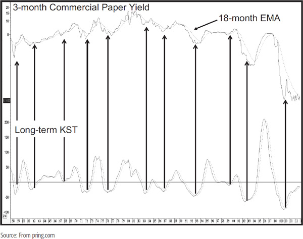
Chart 31.5 shows the rate with an 18-month exponential moving average (EMA) and a long-term Know Sure Thing (KST). Once again, the bullish KST MA crossovers are flagged with the arrows. By and large, a KST MA crossover, when confirmed with an 18-month EMA crossover, has been reasonably reliable. When growth indicator signals are included, the results are even more impressive.
CHART 31.5 3-Month Commercial Paper Yield, 1958–2012, and a Long-Term KST
Movements in the discount rate reflect changes in monetary policy and are, therefore, of key importance to the trend of both short-term interest rates and the equity market. Such action also has a strong psychological influence on both credit and equity markets. This is because the Fed does not reverse policy on a day-to-day or even a week-to-week basis, so a reversal in the trend of the discount rate implies that the trend in market interest rates is unlikely to be reversed for at least several months, and usually far longer. A corporation does not like to cut dividends once they have been raised. In a similar vein, the central bank wishes to create a feeling of continuity and consistency. A change in the discount rate is, therefore, helpful in confirming trends in other rates, which, when taken by themselves, can sometimes give misleading signals because of temporary technical or psychological factors.
Effect on Short-Term Rates Market rates usually lead the discount rate at cyclical turning points. In 2003, the Fed changed the basis on which the discount rate was offered. Consequently, the series plotted in Chart 31.6 represents the post-2003 data spliced to the originally reported series.
CHART 31.6 3-Month Commercial Paper Yield, 1970–2012, and the Adjusted Discount Rate

The objective of the chart is to show that a discount rate cut after a series of hikes acts as confirmation that a new trend of lower rates is under way. The same is true at cyclical or primary-trend bottoms. It is often a good idea to monitor the relationship between the discount rate and its 12-month MA because crossovers almost always signal a reversal in the prevailing trend at a relatively early stage, as flagged by the arrows.
Effect on the Stock Market Since the incorporation of the Federal Reserve System, every bull market peak in equities has been preceded by a rise in the discount rate, with the exception of the Depression, the war years of 1937 and 1939, and more recently, 1976. The leads have varied. In 1973, the discount rate was raised on January 12, 3 days before the bull market high, whereas the 1956 peak was preceded by no fewer than five consecutive hikes.
There is a well-known rule on Wall Street: Three steps and stumble! The rule implies that after three consecutive rate hikes, the equity market is likely to stumble and enter a bear market. The “three steps” rule is, therefore, a recognition that a significant rise in interest rates and tightening in monetary policy have already taken place. Table 31.1 shows the dates when the discount rate was raised for the third time, together with the duration and magnitude of the subsequent decline in equity prices following the third hike.
TABLE 31.1 Discount Rate Highs and Subsequent Stock Market Lows, 1919—2012

Cuts in the rate are equally as important. Generally speaking, as long as the trend of discount rate cuts continues, the primary bull market in stocks should be considered intact. Even after the last cut the market usually possesses enough momentum to extend its advance for a while. Quite often, the last intermediate reaction in the bull market will get underway at the time of or just before the first hike.
Most of the time, the cyclical course of discount rate cuts resembles a series of declining steps, but occasionally it is interrupted by a temporary hike before the downtrend continues. The discount rate low is defined one that occurs after a series of declining steps has taken place, and that either remains unchanged at this low level for at least 15 months or is followed by two or more hikes in 2 different months. In other words, if the series of cuts is interrupted by one hike, the trend is still classified as downward unless the rise occurs after a period of 15 months has elapsed. Only when two hikes in the rate have taken place in a period of less than 15 months is a low considered to have been established. Since the data are available for almost 100 years, they cover both inflationary and deflationary periods and are, therefore, reflective of a number of different economic environments.
Table 31.2 shows that there have been 17 discount rate lows since 1924. On each occasion the market moved significantly higher from the time the rate was cut.
TABLE 31.2 Discount Rate Lows and Subsequent Stock Market Highs, 1924—2012

A discount rate cut is only one indicator, and while it is invariably bullish, the overall technical position is also important. For example, the low in the discount rate usually occurs just after the market has started a bull phase. If the market is long-term overbought, the odds that the ensuing rally will obtain the magnitude and the duration of the average are slim. It should also be noted that while each discount rate low has ultimately been followed by a bull market high, this by no means excludes the risk of a major intermediate correction along the way. Such setbacks occurred in 1934, 1962, and during 1977–1978 and 1998. In the 1977–1978 period the market as measured by the NYSE A/D line did not correct, but moved irregularly higher. Chart 31.7 shows the relationship between the equity market and the discount rate for the decades spanning the turn of the century.
CHART 31.7 S&P Composite, 1970–2012, and the Adjusted Discount Rate

While cuts in the discount rate usually precede market bottoms, this relationship is far less precise than that observed at market tops. Note, for example, that the rate was lowered no fewer than seven times during the 1929–1932 debacle, whereas it was not changed at all during the 1946–1949 bear market.
Bond yield series tend to be very cyclical. We can take advantage of this situation by comparing a series such as Moody’s AAA corporate bonds to an ROC. An example is shown in Chart 31.8, where the arrows show that overbought/oversold crossovers of the 12-month ROC have consistently flashed excellent buy and sell signals. This approach cannot be used as an actual system because offsetting signals may not be given. For example, during the 1940–1981 secular or very long-term uptrend, no buy signals were given between the 1950s and 1981. This contrasts to the post-1981 secular downtrend where several buys were triggered. It is a classic example of how oscillators tend to move and stay at overbought levels during a bull market and reverse the process during bear markets. In this case, the bull market was the secular trend and the overbought readings representedprimary trend peaks.
CHART 31.8 Moody’s AAA Corporate Yield, 1955–2012, and a 12-Month ROC
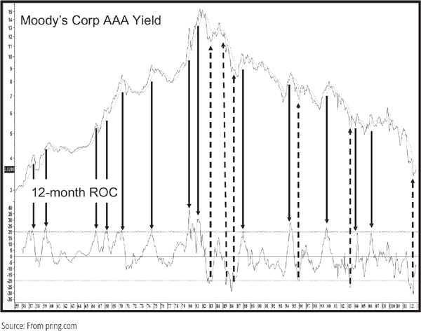
Chart 31.9 expresses a similar idea, except that this time the oscillator is a short-term one, an 8-day MA of a 9-day relative strength indicator (RSI). The arrows above the yield show the primary trend environment. You can see quite clearly that overbought conditions are far more common in the bull phase and oversold during the bear trends. Note also that the 200-day MA can serve as an additional arbitrator of the direction of the primary trend. At the tail end of the chart the oscillator reaches an overbought condition and the yield crosses above its MA, suggesting the probability that a new bull market is under way.
CHART 31.9 The 30-Year Government Bond Yield, 1997–2001, and a Smoothed RSI

Finally, Chart 31.10 compares a perpetual contract of the U.S. Treasury bond futures against two ROC indicators. Between the opening of the year 2000 and the end of the chart, the primary trend was bullish. The four arrows attached to the 10-day ROC indicate oversold or close to oversold conditions. Each was followed by a worthwhile rally. The ellipse in the furthest right part of the chart indicates a failure to respond to an oversold condition and offers the first hint that a new bear market has begun. Several joint trendline breaks in the price and momentum are also indicated on the chart. The adoption of this combination is quite useful because the 10- and 45-day spans are separated by a considerable distance. In this way characteristics not shown by the 10-day series may show up in the 45-day one and vice versa. Of course, it’s even better when all three are indicating a trend reversal, as was the case in April 2000.
CHART 31.10 The 30-Year Government Bond Yield, 1999–2001, Two ROC’s

1. Interest rates influence stock prices because they affect corporate profitability, alter valuation relationships, and influence margin transactions.
2. Interest rates have led stock prices at major turning points in virtually every recorded business cycle.
3. It is the ROC of interest rates, rather than their actual level, that affects equity prices.
4. Short-term interest rates generally have a greater influence on stock prices than long-term ones.
5. Changes in the trend of the discount rate offer strong confirmation that a primary trend change in money-market prices has taken place.
6. Reversals in the trend of the discount rate offer early bird warnings of a change in the primary trend of stock prices.