CHAPTER 3

Working with Data

THE PURPOSE of this chapter is to familiarize the reader with some of the basics of working with data in Julia. As would be expected, much of the focus of this chapter is on or around dataframes, including dataframe functions. Other topics covered include categorical data, input-output (IO), and the split-apply-combine strategy.

3.1  DATAFRAMES

A dataframe is a tabular representation of data, similar to a spreadsheet or a data matrix. As with a data matrix, the observations are rows and the variables are columns. Each row is a single (vector-valued) observation. For a single row, i.e., observation, each column represents a single realization of a variable. At this stage, it may be helpful to explicitly draw the analogy between a dataframe and the more formal notation often used in statistics and data science.

Suppose we observe n realizations x₁, …, x_n of p-dimensional random variables X₁, …, X_n, where X_i = (X_i1, X_i2, …, X_ip)′ for i = 1, …, n. In matrix form, this can be written

$\begin{array}{ll}\mathcal{X}={({\text{X}}_1,{\text{X}}_2,\dots ,{\text{X}}_n)}^{\prime }\hfill & =\left(\begin{array}{c}{\text{X}}_1^{\prime }\\ {\text{X}}_2^{\prime }\\ ⋮\\ {\text{X}}_n^{\prime }\end{array}\right)\hfill \\ \hfill & =\left(\begin{array}{cccc}{X}_{11}& X_{12}& \dots & X_{1p}\\ X_{21}& X_{22}& \dots & X_{2p}\\ ⋮& ⋮& \ddots & ⋮\\ X_{n1}& X_{n2}& \dots & X_{np}\end{array}\right).\hfill \end{array}$

(3.1)

Now, X_i is called a random vector and $\mathcal{X}$ is called an n×p random matrix. A realization of $\mathcal{X}$ can be considered a data matrix. For completeness, note that a matrix A with all entries constant is called a constant matrix.

Consider, for example, data on the weight and height of 500 people. Let x_i = (x_i1,x_i2)′ be the associated observation for the ith person, i = 1, 2, …, 500, where x_i1 represents their weight and x_i2 represents their height. The associated data matrix is then

$\mathcal{X}={({\text{x}}_1,{\text{x}}_2,\dots ,{\text{x}}_{500})}^{\prime }=\left(\begin{array}{c}{\text{x}}_1^{\prime }\\ {\text{x}}_2^{\prime }\\ ⋮\\ {\text{x}}_{500}^{\prime }\end{array}\right)=\left(\begin{array}{cc}{x}_{11}& x_{12}\\ x_{21}& x_{22}\\ ⋮& ⋮\\ x_{500,1}& x_{500,2}\end{array}\right).$

(3.2)

A dataframe is a computer representation of a data matrix. In Julia, the DataFrame type is available through the DataFrames.jl package. There are several convenient features of a DataFrame, including:

•  columns can be different Julia types;

•  table cell entries can be missing;

•  metadata can be associated with a DataFrame;

•  columns can be names; and

•  tables can be subsetted by row, column or both.

The columns of a DataFrame are most often integers, floats or strings, and they are specified by Julia symbols.

## Symbol versus String

fruit = "apple"

println("eval(:fruit): ", eval(:fruit))

# eval(:fruit): apple

println("""eval("apple"): """, eval("apple"))

# eval("apple"): apple

In Julia, a symbol is how a variable name is represented as data; on the other hand, a string represents itself. Note that df[:symbol] is how a column is accessed with a symbol; specifically, the data in the column represented by symbol contained in the DataFrame df is being accessed. In Julia, a DataFrame can be built all at once or in multiple phases.

## Some examples with DataFrames

using DataFrames, Distributions, StatsBase, Random

Random.seed!(825)

N = 50

## Create a sample dataframe

## Initially the DataFrame has N rows and 3 columns

df1 = DataFrame(

  x1 = rand(Normal(2,1), N),

  x2 = [sample(["High", "Medium", "Low"],

           pweights([0.25,0.45,0.30])) for i=1:N],

  x3 = rand(Pareto(2, 1), N)

)

## Add a 4th column, y, which is dependent on x3 and the level of x2 df1[:y] = [df1[i,:x2] == "High" ? *(4, df1[i, :x3]) :

           df1[i,:x2] == "Medium" ? *(2, df1[i, :x3]) :

               *(0.5, df1[i, :x3]) for i=1:N]

A DataFrame can be sliced the same way a two-dimensional Array is sliced, i.e., via df[row_range, column_range]. These ranges can be specified in a number of ways:

•  Using Int indices individually or as arrays, e.g., 1 or [4,6,9].

•  Using : to select indices in a dimension, e.g., x:y selects the range from x to y and : selects all indices in that dimension.

•  Via arrays of Boolean values, where true selects the elements at that index.

Note that columns can be selected by their symbols, either individually or in an array [:x1, :x2].

********

## Slicing DataFrames

println("df1[1:2, 3:4]: ",df1[1:2, 3:4])

println("\ndf1[1:2, [:y, :x1]]: ", df1[1:2, [:y, :x1]])

## Now, exclude columns x1 and x2

keep = setdiff(names(df1), [:x1, :x2])

println("\nColumns to keep: ", keep)

# Columns to keep: Symbol[:x3, :y]

println("df1[1:2, keep]: ",df1[1:2, keep])

In practical applications, missing data is common. In DataFrames.jl, the Missing type is used to represent missing values. In Julia, a singlton occurence of Missing, missing is used to represent missing data. Specifically, missing is used to represent the value of a measurement when a valid value could have been observed but was not. Note that missing in Julia is analogous to NA in R.

In the following code block, the array v2 has type Union{Float64, Missings.Missing}. In Julia, Union types are an abstract type that contain objects of types included in its arguments. In this example, v2 can contain values of missing or Float64 numbers. Note that missings() can be used to generate arrays that will support missing values; specifically, it will generate vectors of type Union if another type is specified in the first argument of the function call. Also, ismissing(x) is used to test whether x is missing, where x is usually an element of a data structure, e.g., ismissing(v2[1]).

## Examples of vectors with missing values

v1 = missings(2)

println("v1: ", v1)

# v1: Missing[missing, missing]

v2 = missings(Float64, 1, 3)

v2[2] = pi

println("v2: ", v2)

# v2: Union{Missing, Float64}[missing 3.14159 missing]

## Test for missing

m1 = map(ismissing, v2)

println("m1: ", m1)

# m1: Bool[true false true]

println("Percent missing v2: ", *(mean([ismissing(i) for i in v2]), 100))

# Percent missing v2: 66.66666666666666

Note that most functions in Julia do not accept data of type Missings.Missing as input. Therefore, users are often required to remove them before they can use specific functions. Using skipmissing() returns an iterator that excludes the missing values and, when used in conjunction with collect(), gives an array of non-missing values. This approach can be used with functions that take non-missing values only.

## calculates the mean of the non-missing values

mean(skipmissing(v2))

# 3.141592653589793

## collects the non-missing values in an array collect(skipmissing(v2))

# 1-element Array{Float64,1}:

# 3.14159

3.2  CATEGORICAL DATA

In Julia, categorical data is represented by arrays of type CategoricalArray, defined in the CategoricalArrays.jl package. Note that CategoricalArray arrays are analogous to factors in R. CategoricalArray arrays have a number of advantages over String arrays in a dataframe:

•  They save memory by representing each unique value of the string array as an index.

•  Each index corresponds to a level.

•  After data cleaning, there are usually only a small number of levels.

CategoricalArray arrays support missing values. The type CategoricalArray{Union{T, Missing}} is used to represent missing values. When indexing/slicing arrays of this type, missing is returned when it is present at that location.

## Number of entries for the categorical arrays

Nca = 10

## Empty array

v3 = Array{Union{String, Missing}}(undef, Nca)

## Array has string and missing values

v3 = [isodd(i) ? sample(["High", "Low"], pweights([0.35,0.65])) :

     missing for i = 1:Nca]

## v3c is of type CategoricalArray{Union{Missing, String},1,UInt32}

v3c = categorical(v3)

## Levels should be ["High", "Low"]

println("1. levels(v3c): ", levels(v3c))

# 1. levels(v3c): ["High", "Low"]

## Reordered levels - does not change the data

levels!(v3c, ["Low", "High"])

println("2. levels(v3c):", levels(v3c))

# 2. levels(v3c): ["Low", "High"]

println("2. v3c: ", v3c)

# 2. v3c: Union{Missing, CategoricalString{UInt32}}

# ["High", missing, "Low", missing, "Low", missing, "High",

# missing, "Low", missing]

Here are several useful functions that can be used with CategoricalArray arrays:

•  levels() returns the levels of the CategoricalArray.

•  levels!() changes the order of the array’s levels.

•  compress() compresses the array saving memory.

•  decompress() decompresses the compressed array.

•  categorical(ca) converts the array ca into an array of type CategoricalArray.

•  droplevels!(ca) drops levels no longer present in the array ca. This is useful when a dataframe has been subsetted and some levels are no longer present in the data.

•  recode(a, pairs) recodes the levels of the array. New levels should be of the same type as the original ones.

•  recode!(new, orig, pairs) recodes the levels in orig using the pairs and puts the new levels in new.

Note that ordered CategoricalArray arrays can be made and manipulated.

## An integer array with three values

v5 = [sample([0,1,2], pweights([0.2,0.6,0.2])) for i=1:Nca]

## An empty string array

v5b = Array{String}(undef, Nca)

## Recode the integer array values and save them to v5b

recode!(v5b, v5, 0 => "Apple", 1 => "Orange", 2=> "Pear")

v5c = categorical(v5b)

print(typeof(v5c))

# CategoricalArray{String,1,UInt32,String,CategoricalString{UInt32},

# Union{}}

print(levels(v5c))

# ["Apple", "Orange", "Pear"]

3.3  INPUT/OUTPUT

The CSV.jl library has been developed to read and write delimited text files. The focus in what follows is on reading data into Julia with CSV.read(). However, as one would expect, CSV.write() has many of the same arguments as CSV.read() and it should be easy to use once one becomes familiar with CSV.read(). Useful CSV.read() parameters include:

•  fullpath is a String representing the file path to a delimited text file.

•  Data.sink is usually a DataFrame but can be any Data.Sink in the DataStreams.jl package, which is designed to efficiently transfer/stream “table-like” data. Examples of data sinks include arrays, dataframes, and databases (SQlite.jl, ODBC.jl, etc.).

•  delim is a character representing how the fields in a file are delimited (| or ,).

•  quotechar is a character used to represent a quoted field that could contain the field or newline delimiter.

•  missingstring is a string representing how the missing values in the data file are defined.

•  datarow is an Int specifying at what line the data starts in the file.

•  header is a String array of column names or an Int specifying the row in the file with the headers.

•  types specifies the column types in an Array of type DataType or a dictionary with keys corresponding to the column name or number and the values corresponding to the columns’ data types.

Before moving into an example using real data, we will illustrate how to change the user’s working directory. R users will be familiar with the setwd() function, which sets the R session’s working directory to a user-defined location. The following code block demonstrates how to set the user’s working directory in Julia using the cd() function. We are using the function homedir() to prepend the path. Note that Windows users have to “Escape” their backslashes when specifying the path.

# Specify working directory

homedir()

# "/Users/paul"

cd("$(homedir())/Desktop")

pwd()

"/Users/paul/Desktop"

# On Windows

# cd("D:\\julia\\projects")

The following code block details how one could go about reading in and cleaning the beer data in Julia. We start by defining some Julia types to store the raw data. This was necessary as the raw data contained missing values in addition to valid entries. The column names that will be used by our dataframe are defined in an array. These same names are used as keys for the dictionary that defines the types for each column. The CSV.jl package is used to read the comma separated value (CSV) data into Julia and store it as a dataframe called df_recipe_raw. From the raw data, a cleaned version of the data is produced, with new columns for a binary outcome and dummy variables produced from the levels of the categorical variables.

using DataFrames, Query, CSV, JLD2, StatsBase, MLLabelUtils, Random

include("chp3_functions.jl")

Random.seed!(24908)

## Types for the files columns

IntOrMiss = Union{Int64,Missing}

FltOrMiss = Union{Float64,Missing}

StrOrMiss = Union{String,Missing}

## define variable names for each column

recipe_header = ["beer_id", "name", "url", "style", "style_id", "size", "og", "fg", "abv", "ibu", "color", "boil_size", "boil_time", "biol_grav", "efficiency", "mash_thick", "sugar_scale", "brew_method", "pitch_rate", "pri_temp", "prime_method", "prime_am"]

## dictionary of types for each column

recipe_types2 = Dict{String, Union}(

  "beer_id" => IntOrMiss,

  "name" => StrOrMiss,

  "url" => StrOrMiss,

  "style" => StrOrMiss,

  "style_id" => IntOrMiss,

  "size" => FltOrMiss,

  "og" => FltOrMiss,

  "fg" => FltOrMiss,

  "abv" => FltOrMiss,

  "ibu" => FltOrMiss,

  "color" => FltOrMiss,

  "boil_size" => FltOrMiss,

  "boil_time" => FltOrMiss,

  "biol_grav" => FltOrMiss,

  "efficiency" => FltOrMiss,

  "mash_thick" => FltOrMiss,

  "sugar_scale" => StrOrMiss,

  "brew_method" => StrOrMiss,

  "pitch_rate" => FltOrMiss,

  "pri_temp" => FltOrMiss,

  "prime_method" => StrOrMiss,

  "prime_am" => StrOrMiss

)

## read csv file

df_recipe_raw = CSV.read("recipeData.csv",

  DataFrame;

  delim = ',',

  quotechar = ' " ',

  missingstring = "N/A",

  datarow = 2,

  header = recipe_header,

  types = recipe_types2,

  allowmissing=: all

)

## Drop columns

delete!(df_recipe_raw, [:prime_method, :prime_am, :url])

#####

## Write the raw data dataframe

JLD2.@save "recipeRaw.jld2" df_recipe_raw

###########################

## Create cleaned version

## Create a copy of the DF

df_recipe = deepcopy(df_recipe_raw)

## exclude missing styles

filter!(row -> !ismissing(row[: style]), df_recipe)

println("-- df_recipe: ",size(df_recipe))

# df_recipe: (73861, 19)

## Make beer categories

df_recipe[:y] = map(x ->

occursin(r"ALE"i, x) || occursin(r"IPA"i, x) || occursin(r"Porter"i, x)

    || occursin(r"stout"i, x) ? 0 :

occursin(r"lager"i, x) || occursin(r"pilsner"i, x) || occursin(r"bock"i, x)

    || occursin(r"okto"i, x) ? 1 : 99,

df_recipe [ : style])

## remove styles that are not lagers or ales

filter!(row -> row[:y] != 99, df_recipe)

## remove extraneous columns

delete!(df_recipe, [:beer_id, :name, : style, :style_id])

## create dummy variables - one-hot-encoding

onehot_encoding!(df_recipe, "brew_method", trace = true)

onehot_encoding!(df_recipe, "sugar_scale")

describe(df_recipe, stats=[:eltype, :nmissing])

delete!(df_recipe, [:brew_method,:sugar_scale])

JLD2.@save "recipe.jld2" df_recipe

The following code block illustrates many of the same steps used to read and clean the food data which is used for our regression examples in Chapters 5 and 7.

using DataFrames, Query, CSV, JLD2, StatsBase, MLLabelUtils, Random

include("chp3_functions.jl")

Random.seed!(24908)

## Types for the file columns

IntOrMiss = Union{Int64,Missing}

FltOrMiss = Union{Float64,Missing}

StrOrMiss = Union{String,Missing}

## define variable names for each column

food_header =

  ["gpa", "gender", "breakfast", "cal_ckn", "cal_day",

   "cal_scone", "coffee", "comfort_food", "comfort_food_reason",

   "comfoodr_code1", "cook", "comfoodr_code2", "cuisine", "diet_current",

   "diet_current_code", "drink", "eating_changes", "eating_changes_coded",

   "eating_changes_coded1", "eating_out", "employment", "ethnic_food",

   "exercise", "father_educ", "father_prof",

   "fav_cuisine", "fav_cuisine_code", "fav_food", "food_child", "fries", "fruit_day",

   "grade_level", "greek_food", "healthy_feeling", "healthy_meal",

   "ideal_diet", "ideal_diet_coded", "income", "indian_food",

   "italian_food", "life_reward", "marital_status", "meals_friend",

   "mom_educ", "mom_prof", "nut_check", "on_campus", "parents_cook",

   "pay_meal_out", "persian_food","self_perception_wgt", "soup", "sports",

   "thai_food", "tortilla_cal", "turkey_cal", "sports_type", "veggies_day",

   "vitamins", "waffle_cal", "wgt"]

## dictionary of types for each column

food_types = Dict{String, Union}(

   "gpa" => FltOrMiss,

   "gender" => IntOrMiss,

   "breakfast" => IntOrMiss,

   "cal_ckn" => IntOrMiss,

   "cal_day" => IntOrMiss,

   "cal_scone" => IntOrMiss,

   "coffee" => IntOrMiss,

   "comfort_food" => StrOrMiss,

   "comfort_food_reason" => StrOrMiss,

   "comfoodr_code1" => IntOrMiss,

   "cook" => IntOrMiss,

   "comfoodr_code2" => IntOrMiss,

   "cuisine" => IntOrMiss,

   "diet_current" => StrOrMiss,

   "diet_current_code" => IntOrMiss,

   "drink" => IntOrMiss,

   "eating_changes" => StrOrMiss,

   "eating_changes_coded" => IntOrMiss,

   "eating_changes_coded1" => IntOrMiss,

   "eating_out" => IntOrMiss,

   "employment" => IntOrMiss,

   "ethnic_food" => IntOrMiss,

   "exercise" => IntOrMiss,

   "father_educ" => IntOrMiss,

   "father_prof" => StrOrMiss,

   "fav_cuisine" => StrOrMiss,

   "fav_cuisine_code" => IntOrMiss,

   "fav_food" => IntOrMiss,

   "food_child" => StrOrMiss,

   "fries" => IntOrMiss,

   "fruit_day" => IntOrMiss,

   "grade_level" => IntOrMiss,

   "greek_food" => IntOrMiss,

   "healthy_feeling" => IntOrMiss,

   "healthy_meal" => StrOrMiss,

   "ideal_diet" => StrOrMiss,

   "ideal_diet_coded" => IntOrMiss,

   "income" => IntOrMiss,

   "indian_food" => IntOrMiss,

   "italian_food" => IntOrMiss,

   "life_reward" => IntOrMiss,

   "marital_status" => IntOrMiss,

   "meals_friend" => StrOrMiss,

   "mom_educ" => IntOrMiss,

   "mom_prof" => StrOrMiss,

   "nut_check" => IntOrMiss,

   "on_campus" => IntOrMiss,

   "parents_cook" => IntOrMiss,

   "pay_meal_out" => IntOrMiss,

   "persian_food" => IntOrMiss,

   "self_perception_wgt" => IntOrMiss,

   "soup" => IntOrMiss,

   "sports" => IntOrMiss,

   "thai_food" => IntOrMiss,

   "tortilla_cal" => IntOrMiss,

   "turkey_cal" => IntOrMiss,

   "sports_type" => StrOrMiss,

   "veggies_day" => IntOrMiss,

   "vitamins" => IntOrMiss,

   "waffle_cal" => IntOrMiss,

   "wgt" => FltOrMiss

)

## read csv file

df_food_raw = CSV.read("food_coded.csv",

   DataFrame;

   delim = ',',

   quotechar = '"',

   missingstrings = ["nan", "NA", "na", ""],

   datarow = 2,

   header = food_header,

   types = food_types,

   allowmissing=: all

)

## drop text fields which are not coded fields

delete!(df_food_raw, [:comfort_food, :comfort_food_reason, :comfoodr_code2,

   :diet_current, :eating_changes, :father_prof, :fav_cuisine, :food_child,

   :healthy_meal, :ideal_diet, :meals_friend, :mom_prof, :sports_type

])

## Change 1/2 coding to 0/1 coding

df_food_raw[:gender] = map(x -> x - 1, df_food_raw[:gender])

df_food_raw[:breakfast] = map(x -> x - 1, df_food_raw[:breakfast])

df_food_raw[:coffee] = map(x -> x - 1, df_food_raw[:coffee])

df_food_raw[:drink] = map(x -> x - 1, df_food_raw[:drink])

df_food_raw[:fries] = map(x -> x - 1, df_food_raw[:fries])

df_food_raw[:soup] = map(x -> x - 1, df_food_raw[:soup])

df_food_raw[:sports] = map(x -> x - 1, df_food_raw[:sports])

df_food_raw[:vitamins] = map(x -> x - 1, df_food_raw[:vitamins])

JLD2.@save "food_raw.jld2" df_food_raw

###########################

## Create cleaned version

## Create a copy of the DF

df_food = deepcopy(df_food_raw)

println("- df_food size: ", size(df_food))

# - df_food size: (125, 48)

## generate dummy variables

## used string array bc onehot_encoding!() takes a string

change2_dv = ["cal_ckn", "cal_day", "cal_scone", "comfoodr_code1",

   "cook", "cuisine", "diet_current_code", "eating_changes_coded",

   "eating_changes_coded1", "eating_out", "employment", "ethnic_food",

   "exercise", "father_educ", "fav_cuisine_code", "fav_food", "fruit_day",

   "grade_level", "greek_food", "healthy_feeling", "ideal_diet_coded",

   "income", "indian_food", "italian_food", "life_reward", "marital_status",

   "mom_educ", "nut_check", "on_campus", "parents_cook", "pay_meal_out",

   "persian_food", "self_perception_wgt", "thai_food", "tortilla_cal",

   "turkey_cal", "veggies_day", "waffle_cal"]

println("-- onehotencoding()")

for i in change2_dv

   println("i: ", i)

   onehot_encoding!(df_food, i)

   delete!(df_food, Symbol(i))

end

## remove NaNs

df_food[:gpa] =

   collect(FltOrMiss, map(x -> isnan(x)?missing:x, df_food[:gpa]))

df_food[:wgt] =

   collect(FltOrMiss, map(x -> isnan(x)?missing:x, df_food[:wgt]))

## remove missing gpa

filter!(row -> !ismissing(row[:gpa]), df_food)

println("--- df_food: ", size(df_food))

# --- df_food: (121, 214)

JLD2.@save "food.jld2" df_food

3.4  USEFUL DATAFRAME FUNCTIONS

There are several dataframe functions that have not been mentioned yet but that are quite useful:

•  eltype() provides the types for each element in a DataFrame.

•  head(df, n) displays the top n rows.

•  tail(df, n) displays the bottom n rows.

•  size(df) returns a tuple with the dimensions of the DataFrame.

•  size(df, 1) returns the number of columns.

•  size(df, 2) returns the number of rows.

•  describe(df) returns statistical summary measures along with column types for each column in the df.

•  colwise(f, df) applies function f to the columns in df.

•  delete!(df, col_symbol) removes one or more columns, where columns are referenced by a symbol or an array of symbols, e.g., :x1 or [:x1, :x2].

•  rename!(df, :old_name => :new_name) uses a Pair data structure to specify the existing name and its new name. The Pair data structure can be created dynamically:

rename!(df1, o => n for (o, n) = zip([:x1, :x2, :x3, :y],

  [:X1, :X2, :X3, :Y]))

•  filter(f, df) filters the rows in dataframe df using the anonymous function f and returns a copy of df with the rows filtered by removing elements where f is false.

•  filter!(f, df) updates the dataframe df; note that no copy is created.

## remove rows where the style column is missing.

filter!(row -> !ismissing(row[:style]), df_recipe)

•  push!(df, item) adds one or more items item to the dataframe df that are not already in a dataframe.

•  append!(df1, df2) adds dataframe df2 to dataframe df1.

Several functions listed here have clear analogues in R. For example, the describe() function in Julia is similar to the summary() function in R. Similarly, the size() function in Julia is similar to the dim() function in R.

## using the dataframe previously defined

describe(df1[:X1])

# Summary Stats:

# Mean:            2.078711

# Minimum:        -0.229097

# 1st Quartile:   1.262696

# Median:         2.086254

# 3rd Quartile:   2.972752

# Maximum:        4.390025

# Length:         50

# Type:           Float64

## number of rows and columns of df_1

size(df1)

# (50, 4)

3.5  SPLIT-APPLY-COMBINE STRATEGY

Often data scientists need to extract summary statistics from the data in dataframes. The split-apply-combine (SAC) strategy is a convenient way to do this. This strategy for data analysis was outlined by Wickham (2011) and is implemented as the plyr package (Wickham, 2016) for R. The strategy involves partitioning the dataset into groups and administering some function to the data in each group and then recombining the results. Julia implements this strategy with one of:

•  by(df, cols, f),

•  groupby(df, cols, skipmissing = false), or

•  aggregate(df, cols, f).

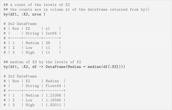
The function by(df, cols, f) is used to apply function f to the dataframe df, partitioning by the column(s) cols in the dataframe. The function by() takes the following arguments:

•  df is the dataframe being analyzed.

•  cols is the columns making up the groupings.

•  f is the function being applied to the grouped data.

The function by(df, cols, f) returns a DataFrame of the results.

The function groupby(df, cols, skipmissing = false) splits a dataframe df into sub-dataframes by rows and takes the following arguments:

•  df is the DataFrame to be split.

•  cols is the columns by which to split up the dataframe.

•  skipmissing determines if rows in cols should be skipped if they contain missing entries and returns a grouped DataFrame object that can be iterated over, returning sub-dataframes at each iteration.

The function groupby(df, cols, skipmissing = false) returns a grouped DataFrame object, each sub-dataframe in this object is one group, i.e., a DataFrame, and the groups are accessible via iteration.

## print the summary stats for x3 in each partition

for part in groupby(df1, :X2, sort=true)

   println(unique(part[:X2]))

   println(summarystats(part[:X3]))

end

# ["High"]

# Summary Stats:

# Mean:         2.004051

# Minimum:      1.011101

# 1st Quartile: 1.361863

# Median:       1.820108

# 3rd Quartile: 2.383068

# Maximum:      4.116220

#

# ["Low"]

# …

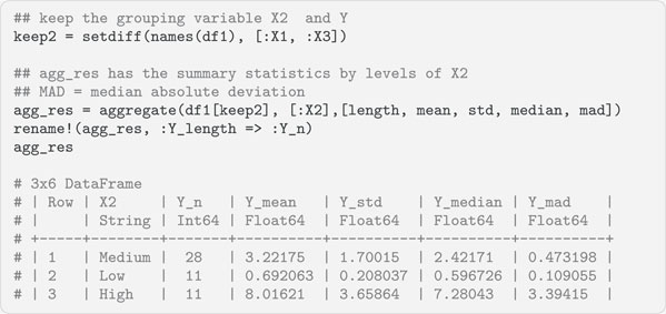
The function aggregate(df, cols, f) splits a dataframe df into sub-dataframes by rows and takes the following arguments:

•  df is the dataframe being analyzed.

•  cols are the columns that make up the groupings.

•  f is the function to apply to the remaining data. Multiple functions can be specified as an array, e.g., [sum, mean].

The function aggregate(df, cols, f) returns a DataFrame.

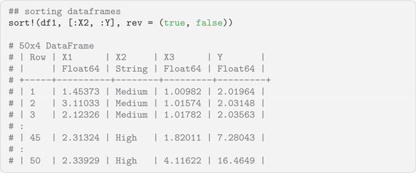
Often dataframes need to be sorted. This can be accomplished with the sort!() function. The ! in the function names indicates it will sort the object in place and not make a copy of it. When sorting dataframes, users will most often want to select the columns to sort by and the direction to sort them (i.e., ascending or descending). To accomplish this, the sort!() function takes the following arguments:

•  df is the dataframe being sorted.

•  cols is the dataframe columns to sort. These should be column symbols, either alone or in an array.

•  rev is a Boolean value indicating whether the column should be sorted in descending order or not.

3.6  QUERY.JL

Query.jl is a Julia package used for querying Julia data sources. These data sources include the ones we have mentioned, such as dataframes and data streams such as CSV. They can also include databases via SQLite and ODBS, and time series data through the TimeSeries.jl framework. Query.jl can interact with any iterable data source supported through the IterableTables.jl package. It has many features that will be familiar to users of the dplyr package (Wickham et al., 2017) in R.

At the time of writing, Query.jl is heavily influenced by the query expression portion of the C# Language-INtegrated Query (LINQ) framework (Box and Hejlsberg, 2007). LINQ is a component of the .NET framework that allows the C# language to natively query data sources in the form of query expressions. These expressions are comparable to SQL statements in a traditional database and allow filtering, ordering and grouping operations on data sources with minimal code. The LINQ framework allows C# to query multiple data sources using the same query language. Query.jl gives data scientists this capability in Julia, greatly simplifying their work.

The following code block shows the basic structure of a Query.jl query statement. The @from statement is provided by the package which specifies how the query will iterate over the data source. This is done in the same way a for loop iterates over a data source, using a range variable, often i, the in operator and the data source name. There can be numerous query statements where <statements> is written in the below code block, each one would be separated by a new line. The result of the query is stored in the x_obj object which can be a number of different data sinks, including dataframes and CSV files.

## Pseudo code for a generic Query.jl statement

## the query statements in <statements> are separated by \n

x_obj = @from <range_var> in <data_source> begin

  <statements>

end

We will start our overview of Query.jl features with a simple example using the beer data. The following code block shows how to filter rows with the @where statement, select columns with the @select statement, and return the result as a DataFrame object with the @collect statement.

using Query

## select lagers (y ==1) and pri_temp >20

x_obj = @from i in df_recipe begin

  @where i.y == 1 && i.pri_temp > 20

  @select {i.y, i.pri_temp, i.color}

  @collect DataFrame

end

typeof(x_obj)

# DataFrame

names(x_obj)

# Symbol[3]

# :y

# :pri_temp

# :color

size(x_obj)

# (333, 3)

Notice that the @where and @select statements use the iteration variable i to reference the columns in the dataframe. The dataframe df_recipe is the data source for the query. The @collect macro returns the result of the query as an object of a given format. The formats available are called data sinks and include arrays, dataframes, dictionaries or any data stream available in DataStreams.jl, amongst others.

The @where statement is used to filter the rows of the data source. It is analogous to the filter! function described in Section 3.3. The expression following @where can be any arbitrary Julia expression that evaluates to a Boolian value.

The @select statement can use named tuples, which are integrated into the base language. They are tuples that allow their elements to be accessed by an index or a symbol. A symbol is assigned to an element of the tuple, and @select uses these symbols to construct column names in the data sink being used. Named tuples are illustrated in the following code block. The second element is accessed via its symbol, unlike a traditional tuple which would only allow access via its index (e.g., named_tup[2]). Named tuples can be defined in a @select statement in two ways, using the traditional (name = value) syntax or the custom Query.jl syntax {name = value}.

## named tuple - reference property by its symbol

named_tup = (x = 45, y = 90)

typeof(named_tup)

# NamedTuple{(:x, :y),Tuple{Int64,Int64}}

named_tup[:y]

# 90

The next code block shows how to query a dataframe and return different arrays. The first query filters out the rows of the dataframe, uses the get() function to extract the values of the colour column and returns them as an array. Arrays are returned when no data sink is specified in the @collect statement. The second query selects two columns of the dataframe and returns an array. This array is an array of named tuples. To create a two-dimensional array of floating point values, additional processing is required. The loop uses the arrays’ indices and the symbols of the named tuple to populate the array of floats.

## Returns an array of Float64 values

a1_obj = @from i in df_recipe begin

  @where i.y == 1 && i.color <= 5.0

  @select get(i.color) #Float64[1916]

  @collect

end

a1_obj

# 1898-element Array{Float64,1}:

# 3.3

# 2.83

# 2.1

## Returns a Named Tuple array. Each row is a NT with col and ibu values

a2_obj = @from i in df_recipe begin

  @where i.y == 1 && i.color <= 5.0

  @select {col = i.color, ibu = i.ibu}

  @collect

end

a2_obj

# 1898-element Array{NamedTuple{(:col, :ibu),Tuple{DataValues.DataValue{

# Float64},DataValues.DataValue{Float64}}},1}:

# (col = DataValue{Float64}(3.3), ibu = DataValue{Float64}(24.28))

# (col = DataValue{Float64}(2.83), ibu = DataValue{Float64}(29.37))

## Additional processing to return an Array of floats

N = size(a2_obj)[1]

a2_array =zeros(N, 2)

for (i,v) in enumerate(a2_obj)

  a2_array[i, 1] = get(a2_obj[i][:col],0)

  a2_array[i, 2] = get(a2_obj[i][:ibu],0)

end

a2_array

# 1898x2 Array{Float64,2}:

# 3.3 24.28

# 2.83 29.37

Another common scenario is querying a data structure and returning a dictionary. This can be accomplished in Query.jl by specifying the Dict type in the @collect statement. In addition to this, the @select statement should include a pair expression, the first variable being the dictionary’s key, the second being its value.

## data sink is dictionary

## select statement creates a Pair

dict_obj = @from i in df_recipe begin

  @where i.y == 1 && i.color <= 5.0

  @select i.id => get(i.color)

  @collect Dict

end

typeof(dict_obj)

# Dict{String,Float64}

dict_obj

# Dict String -> Float64 with 1898 entries

# "id16560" -> 3.53

# "id31806" -> 4.91

# "id32061" -> 3.66

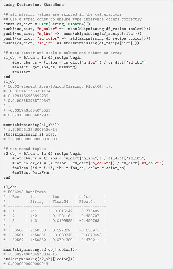
In Query.jl, the @let statement can be used to create new variables in a query, known as range variables. The @let statement is used to apply a Julia expression to the elements of the data source and writes them to a data sink. The following code block details how to do this in the case where the objective is to mean centre and scale each column to have a mean of 0 and a standard deviation of 1. The @let statement can have difficulty with type conversion, so we define a constant dictionary with specified types. We store the column means and standard deviations here. The @let statement uses the dictionary values to do the centering and scaling.

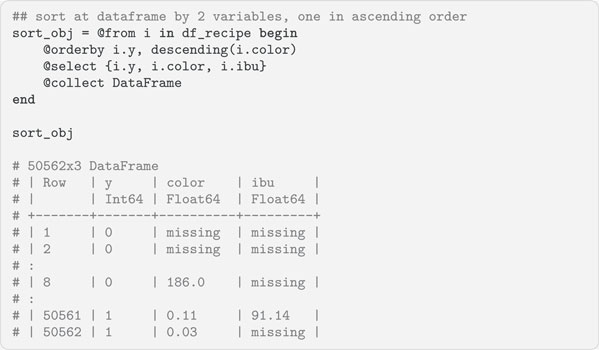
Sorting is a common task when working with data. Query.jl provides the @orderby statement to do sorting. It sorts the data source by one or more variables and the default sort order is ascending. If multiple variables are specified, they are separated by commas and the data source is sorted first by the initial variable in the specification. The descending() function can be used to change each variable’s sorting order. Sorting is detailed in the following code block.

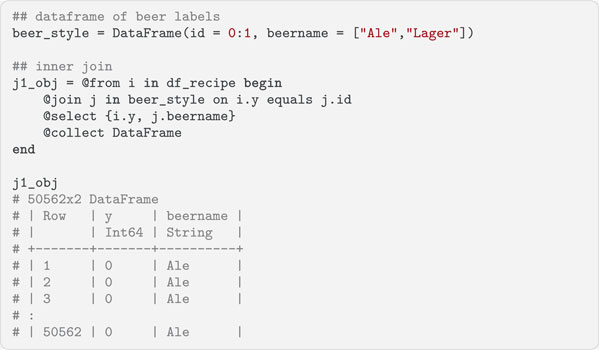
When working with multiple datasets, combining them is often necessary before the data can be analyzed. The @join statement is used to do this and implements many of the traditional database joins. We will illustrate an inner join in the next code block. Left outer and group joins are also available. The @join statement creates a new range variable j for the second data source and uses id as the key. This key is compared to a key from the first data source y and matches are selected. Inner joins return all the rows that share the specified key values in both data sources, which in this case is all the rows in df_recipe.

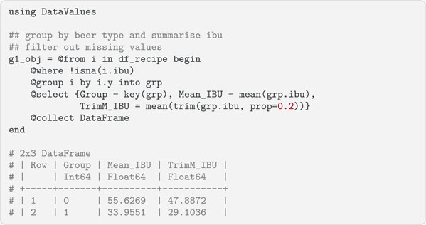
When processing data, it is often necessary to group the data into categories and calculate aggregate summaries for these groups. Query.jl facilitates this with the @group statement. It groups data from the data source by levels of the specified columns into a new range variable. This range variable is used to aggregate the data. In the following code block, we group the df_recipe dataframe by the beer categories y. The new range variable is called grp and is used in the @select statement to specify which data are used. The @where statement filters out the missing values in the IBU variable. In the query, missing values are represented as instances of the Query.jl data type DataValue. Consequently, isna() from the DataValues.jl package is used to filter them out and not ismissing(). The data for each group is aggregated by its mean and trimmed mean values.