© Orhan Gazi Yalçın 2021

O. G. YalçınApplied Neural Networks with TensorFlow 2https://doi.org/10.1007/978-1-4842-6513-0_12

12. Generative Adversarial Network

Orhan Gazi Yalçın¹  

(1)

Istanbul, Turkey

 

Generative adversarial networks (GANs) are a type of deep learning model designed by Ian Goodfellow and his colleagues in 2014.

The invention of GANs has occurred pretty unexpectedly. The famous researcher, then, a PhD fellow at the University of Montreal, Ian Goodfellow, landed on the idea when he was discussing with his friends – at a friend's going away party – about the flaws of the other generative algorithms. After the party, he came home with high hopes and implemented the concept he had in mind. Surprisingly, everything went as he hoped in the first trial, and he successfully created the generative adversarial networks (shortly, GANs).

According to Yann LeCun, the director of AI research at Facebook and a professor at New York University, GANs are “the most interesting idea in the last 10 years in machine learning.”

Method

In a GAN architecture, there are two neural networks (a generator and a discriminator) competing with each other in a game. After being exposed to a training set, the generator learns to generate new samples with similar characteristics. The discriminator, on the other hand, tries to figure out if the generated data is authentic or manufactured. Through training, the generator is forced to generate near-authentic samples so that the discriminator cannot differentiate them from the training data. After this training, we can use the generator to generate very realistic samples such as images, sounds, and text.

GANs are initially designed to address unsupervised learning tasks. However, recent studies showed that GANs show promising results in supervised, semi-supervised, and reinforcement learning tasks as well.

Architecture

As mentioned earlier, there are two networks forming a generative adversarial network: a generator network and a discriminator network. These two networks are connected to each other with a latent space where all the magic happens. In other words, we use the output of the generator network as the input in the discriminator network. Let’s take an in-depth look at the generative and discriminative networks to truly understand how GANs function; see Figure 12-1:

Figure 12-1

A Visualization of a Generative Adversarial Network

GAN Components

Generative Network

A generator network takes a fixed-length random vector (starting with random noise) and generates a new sample. It uses a Gaussian distribution to generate new samples and usually starts with a one-dimensional layer, which is reshaped into the shape of the training data samples in the end. For example, if we use the MNIST dataset to generate images, the output layer of the generator network must correspond to the image dimensions (e.g., 28 x 28 x 1). This final layer is also referred to as latent space or vector space.

Discriminator Network

A discriminator network works in a relatively reversed order. The output of the generative network is used as input data in the discriminator network (e.g., 28 x 28 x 1). The main task of a discriminator network is to decide if the generated sample is authentic or not. Therefore, the output of a discriminator network is provided by a single neuron dense layer outputting the probability (e.g., 0.6475) of the authenticity of the generated sample.

Latent Space

Latent space (i.e.,vector space) functions as the generator network's output and the discriminator network's input. The latent space in a generative adversarial model usually has the shape of the original training dataset samples. Latent Space tries to catch the characteristic features of the training dataset so that the generator may successfully generate close to authentic samples.

A Known Issue: Mode Collapse

During the training of the generative adversarial networks, we often encounter with the “mode collapse” issue. Mode collapse basically refers to the failure to generalize correctly or, in other words, failure to learn the meaningful characteristics for successful sample generation. Mode collapse may be in the form of failure to learn altogether or failure to learn partial features. For example, when we work with the MNIST dataset (handwritten digits from 0 to 9), due to mode collapse issue, our GAN may never learn to generate some of the digits. There are two potential explanations for mode collapse:

• Weak discriminative network

• Wrong choice of objective function

Therefore, playing around with the size and depth of our network, as well as with objective function, may fix the issue.

Final Notes on Architecture

It is essential to maintain healthy competition between generator and discriminator networks to build useful GAN models. As long as these two networks work against each other to perfect their performances, you can freely design the internal structure of these networks, depending on the problem. For example, when you are dealing with sequence data, you can build two networks with LSTM and GRU layers as long as one of them acts as a generator network, whereas the other acts as a discriminator network. Another example would be our case study. When to generate images with GANS, we add our networks a number of Convolution or Transposed Convolution layers since they decrease the computational complexity of the image data.

Applications of GANs

There are a number of areas where the GANs are currently in use which may be listed as follows:

• Fashion, art, and advertising

• Manufacturing and R&D

• Video games

• Malicious applications and deep fake

• Other applications

Art and Fashion

Generative adversarial networks are capable of “generating” samples. So, they are inherently creative. That’s why one of the most promising fields for generative adversarial networks is art and fashion. With well-trained GANs, you can generate paintings, songs, apparels, and even poems. In fact, a painting generated by Nvidia’s StyleGAN network, “Edmond de Belamy, from La Famille de Belamy,” was sold in New York for $432,500. Therefore, you may clearly see how GAN has the potential to be used in the art world.

Manufacturing, Research, and R&D

GANs can be used to predict computational bottlenecks in scientific research projects as well as in industrial applications.

GAN networks can also be used to increase the definition of images based on statistical distributions. In other words, GANs can predict the missing pieces using statistical distributions and generate suitable pixel values, which would increase the quality of the images taken by telescopes or microscopes.

Video Games

GANs may be used to obtain more precise and sharper images using small definition images. This ability may be used to make old games more appealing to new generations.

Malicious Applications and Deep Fake

GANs may be used to generate close-to-authentic fake social profiles or fake videos of celebrities. For example, a GAN algorithm may be used to fabricate fake evidence to frame someone. Therefore, there are a number of malicious GAN applications and also a number of GANs to detect the samples generated by the malicious GANs and label them as fake.

Miscellaneous Applications

Apart from the preceding use cases, GANs are used with the following purposes:

• For early diagnosis in the medical industry

• To generate photorealistic images in architecture and internal design industries

• To reconstruct three-dimensional models of objects from images

• For image manipulation such as aging

• To generate protein sequences which may be used in cancer studies

• To reconstruct a person’s face by using their voice.

The generative adversarial network applications are vast and limitless, and it is a very hot topic in the artificial intelligence community. Now that we covered the basics of generative adversarial networks, we can start working on our case study. Note that we will do our own take from deep convolutional GAN tutorial released by the TensorFlow team.¹

Case Study | Digit Generation with MNIST

In this case study, step by step, we build a generative adversarial network (GAN), which is capable of generating handwritten digits (0 to 9). To be able to complete this task, we need to build a generator network as well as a discriminator network so that our generative model can learn to trick the discriminator model, which inspects what the generator network manufactures. Let’s start with our initial imports.

Initial Imports

As we always do in our case studies, we make some initial imports, which are used throughout different cells of our Colab notebook. The following lines import TensorFlow, relevant TensorFlow layer objects, and Matplotlib:

import tensorflow as tf

from tensorflow.keras.layers import(Dense,

                                 BatchNormalization,

                                 LeakyReLU,

                                 Reshape,

                                 Conv2DTranspose,

                                 Conv2D,

                                 Dropout,

                                 Flatten)

import matplotlib.pyplot as plt

In the upcoming parts, we also use other libraries such as os, time, IPython.display, PIL, glob, and imageio, but to keep them relevant with the context, we only import them when we will use them.

Load and Process the MNIST Dataset

We already covered the details of the MNIST dataset a few times. It is a dataset of handwritten digits with 60,000 training and 10,000 test samples. If you want to know more about the MNIST dataset, please refer to Chapter 7.

Since this is an unsupervised learning task, we only need the features, and therefore we don’t save the label arrays. Let’s import the dataset with the following lines:

# underscore to omit the label arrays

(train_images, train_labels), (_, _) = tf.keras.datasets.mnist.load_data()

Then, we reshape our train_images to have a fourth dimension and normalize it (in range of -1 to 1) with the following code:

train_images = train_images.reshape(train_images.shape[0], 28, 28, 1).astype('float32')

train_images = (train_images - 127.5) / 127.5 # Normalize the images to [-1, 1]

Then, we set a BUFFER_SIZE for shuffling and a BATCH_SIZE for processing the data in batches. Then, we call the following function to convert our NumPy array into a TensorFlow Dataset object:

# Batch and shuffle the data

train_dataset = tf.data.Dataset.from_tensor_slices(train_images).shuffle(BUFFER_SIZE).batch(BATCH_SIZE)

Now our data is processed and cleaned. We can move on to the model-building part.

Build the GAN Model

As opposed to the other case studies, the model-building part of this case study is slightly more advanced. We need to define custom loss, training step, and training loop functions. It may be a bit more challenging to grasp what is happening. But I try to add as much comment as possible to make it easier for you. Also, consider this case study as a path to becoming an advanced machine learning expert. Besides, if you really pay attention to the comments, it is much easier than how it looks.

Generator Network

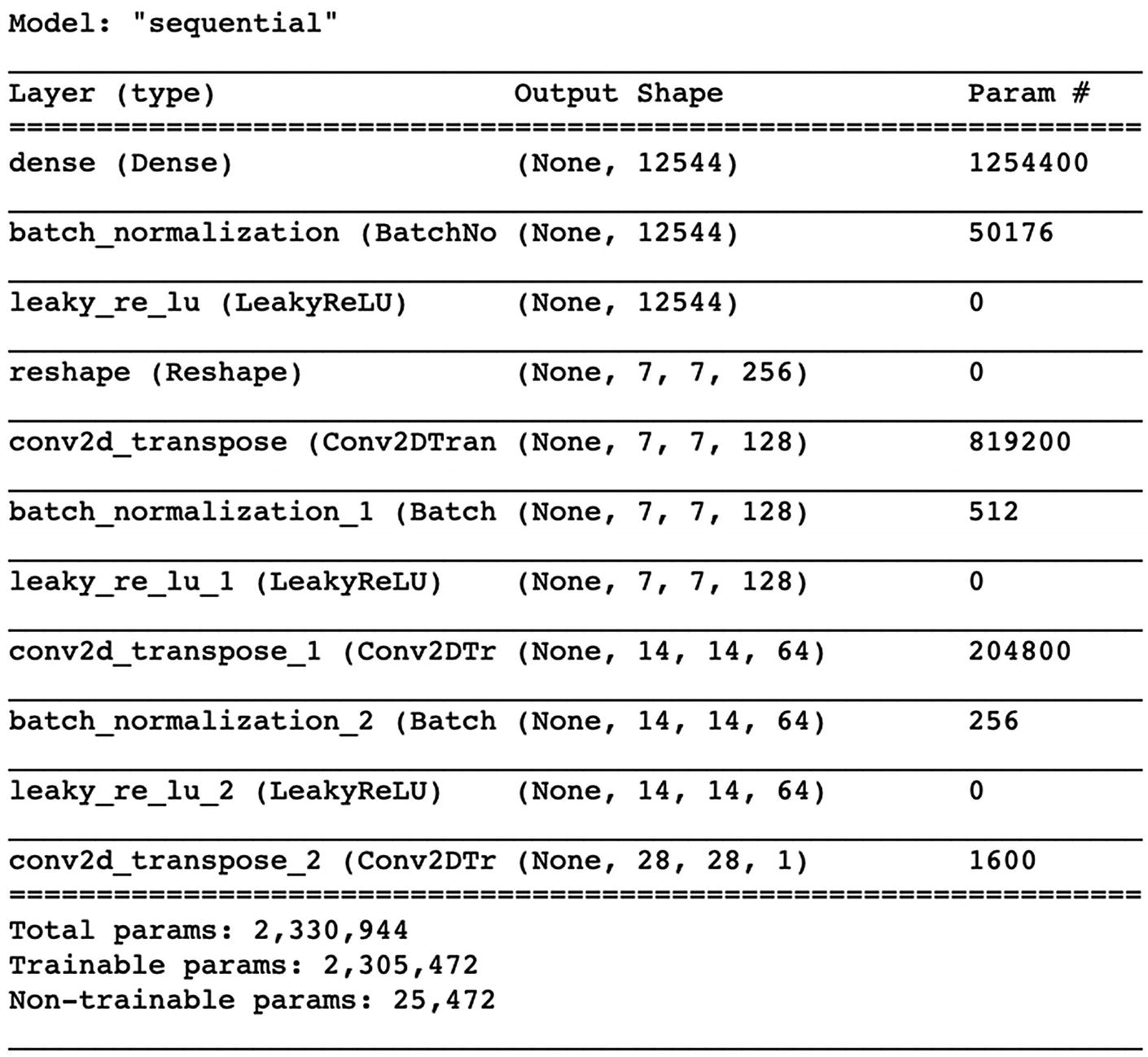
As part of our GAN network, we first build a generator with Sequential API. The generator would accept a one-dimensional input with 100 data points and slowly converts it into an image data of 28 x 28 pixels. Since we use this model to generate images from one-dimensional input, using Transposed Convolution layers is the best option. Transposed Convolution layers work just the opposite of the Convolution layer. They increase the definition of image data. We also take advantage of Batch Normalization and Leaky ReLU layers after using Transposed Convolution layers. The following code defines this network for us:

def make_generator_model():

  model = tf.keras.Sequential()

  model.add(Dense(7*7*256, use_bias=False, input_shape=(100,)))

  model.add(BatchNormalization())

  model.add(LeakyReLU())

  model.add(Reshape((7, 7, 256)))

  assert model.output_shape == (None, 7, 7, 256) # Note: None is the batch size

  model.add(Conv2DTranspose(128, (5, 5), strides=(1, 1), padding="same", use_bias=False))

  assert model.output_shape == (None, 7, 7, 128)

  model.add(BatchNormalization())

  model.add(LeakyReLU())

  model.add(Conv2DTranspose(64, (5, 5), strides=(2, 2), padding="same", use_bias=False))

  assert model.output_shape == (None, 14, 14, 64)

  model.add(BatchNormalization())

  model.add(LeakyReLU())

  model.add(Conv2DTranspose(1, (5, 5), strides=(2, 2), padding="same", use_bias=False, activation="tanh"))

  assert model.output_shape == (None, 28, 28, 1)

  return model

We can declare our network with the following code:

generator = make_generator_model()

Let’s take a look at the summary of our generator network in Figure 12-2:

generator.summary()

Output:

Figure 12-2

The Summary of Our Generator Network

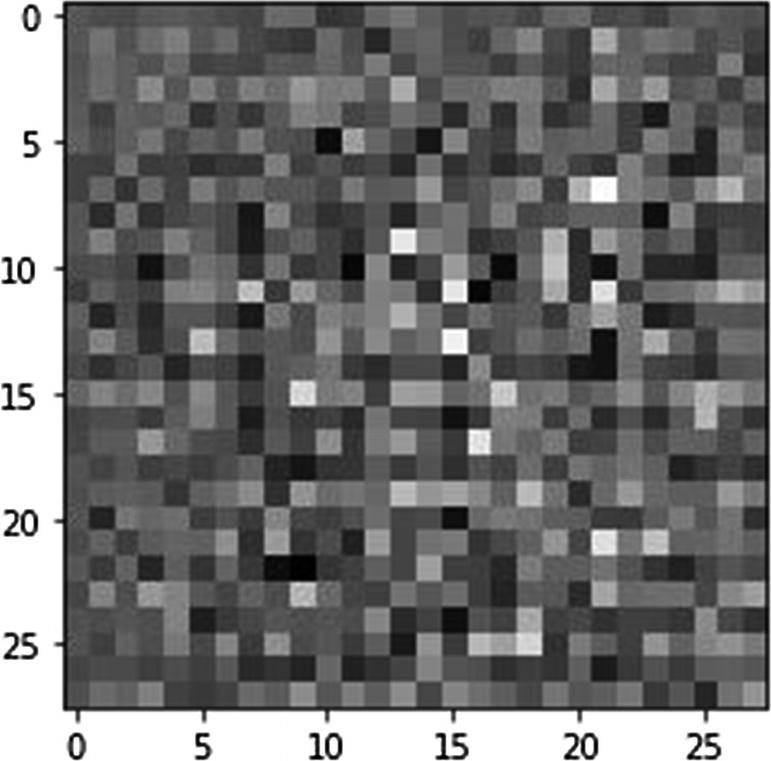
And generate and plot a sample using our untrained generator network with the following code:

# Create a random noise and generate a sample

noise = tf.random.normal([1, 100])

generated_image = generator(noise, training=False)

# Visualize the generated sample

plt.imshow(generated_image[0, :, :, 0], cmap="gray")

Output is shown in Figure 12-3:

Figure 12-3

An Example of the Randomly Generated Sample Without Training

Discriminator Network

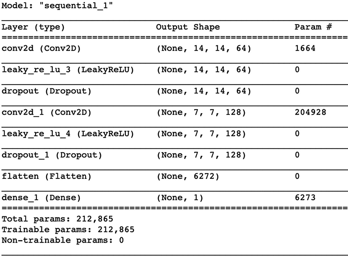
After the generator network, we should build a discriminator network to inspect the samples generated by the generator. Our discriminator network must decide on the probability of the fakeness of the generated images. Therefore, it takes the generated image data (28 x 28) and outputs a single value. For this task, we use Convolution layers supported by Leaky ReLU and Dropout layers. Flatten layers convert two-dimensional data into one-dimensional data, and Dense layer is used to convert the output into a single value. The following lines define the function for our discriminator network:

def make_discriminator_model():

  model = tf.keras.Sequential()

  model.add(Conv2D(64, (5, 5), strides=(2, 2), padding="same", input_shape=[28, 28, 1]))

  model.add(LeakyReLU())

  model.add(Dropout(0.3))

  model.add(Conv2D(128, (5, 5), strides=(2, 2), padding="same"))

  model.add(LeakyReLU())

  model.add(Dropout(0.3))

  model.add(Flatten())

  model.add(Dense(1))

  return model

We can create the discriminator network by calling the function:

discriminator = make_discriminator_model()

And we can see the summary of our discriminator network with the following code (see Figure 12-4 for the output):

discriminator.summary()

Output:

Figure 12-4

The Summary of Our Discriminator Network

If we use the discriminator network, we can actually decide if our randomly generated image is authentic enough or not:

decision = discriminator(generated_image)

print (decision)

Output:

tf.Tensor([[-0.00108097]], shape=(1, 1), dtype=float32)

As you can see, our output is less than zero, and we can conclude that this particular sample generated by the untrained generator network is fake.

Configure the GAN Network

As part of our model configuration, we need to set loss functions for both the generator and the discriminator. In addition, we need to set separate optimizers for both of them as well.

Loss Function

We start by creating a Binary Crossentropy object from tf.keras.losses module. We also set from_logits parameter to true. After creating the object, we fill them with custom discriminator and generator loss functions.

Our discriminator loss is calculated as a combination of (i) the discriminator’s predictions on real images to an array of ones and (ii) its predictions on generated images to an array of zeros.

Our generator loss is calculated by measuring how well it was able to trick the discriminator. Therefore, we need to compare the discriminator’s decisions on the generated images to an array of ones.

The following lines do all of these:

# This method returns a helper function to compute cross entropy loss

cross_entropy = tf.keras.losses.BinaryCrossentropy(from_logits=True)

def discriminator_loss(real_output, fake_output):

  real_loss = cross_entropy(tf.ones_like(real_output), real_output)

  fake_loss = cross_entropy(tf.zeros_like(fake_output), fake_output)

  total_loss = real_loss + fake_loss

  return total_loss

def generator_loss(fake_output):

  return cross_entropy(tf.ones_like(fake_output), fake_output)

Optimizer

We also set two optimizers separately for generator and discriminator networks. We can use the Adam object from tf.keras.optimizers module. The following lines set the optimizers:

generator_optimizer=tf.keras.optimizers.Adam(1e-4)

discriminator_optimizer=tf.keras.optimizers.Adam(1e-4)

Set the Checkpoint

Training the GAN network takes longer than other networks due to the complexity of the network. We have to run the training for at least 50–60 epochs to generate meaningful images. Therefore, setting checkpoints is very useful to use our model later on.

By using the os library, we set a path to save all the training steps with the following lines:

import os

checkpoint_dir = './training_checkpoints'

checkpoint_prefix=os.path.join(checkpoint_dir, "ckpt")

checkpoint = tf.train.Checkpoint(

  generator_optimizer=generator_optimizer,

  discriminator_optimizer=discriminator_optimizer,

  generator=generator,

  discriminator=discriminator)

Train the GAN Model

Let’s create some of the variables with the following lines:

EPOCHS = 60

# We will reuse this seed overtime (so it's easier)

# to visualize progress in the animated GIF)

noise_dim = 100

num_examples_to_generate = 16

seed = tf.random.normal([num_examples_to_generate, noise_dim])

Our seed is the noise that we use to generate images on top of. The following code generates a random array with normal distribution with the shape (16, 100).

The Training Step

This is the most unusual part of our model: We are setting a custom training step. After defining the custom train_step() function by annotating the tf.function module, our model will be trained based on the custom train_step() function we defined.

The following code with excessive comments are for the training step. Please read the comments carefully.

# tf.function annotation causes the function

# to be "compiled" as part of the training

@tf.function

def train_step(images):

  # 1 - Create a random noise to feed it into the model

  # for the image generation

  noise = tf.random.normal([BATCH_SIZE, noise_dim])

  # 2 - Generate images and calculate loss values

  # GradientTape method records operations for automatic differentiation.

  with tf.GradientTape() as gen_tape, tf.GradientTape() as disc_tape:

    generated_images = generator(noise, training=True)

    real_output = discriminator(images, training=True)

    fake_output = discriminator(generated_images, training=True)

    gen_loss = generator_loss(fake_output)

    disc_loss = discriminator_loss(real_output, fake_output)

  # 3 - Calculate gradients using loss values and model variables

  # "gradient" method computes the gradient using

  # operations recorded in context of this tape (gen_tape and disc_tape).

  # It accepts a target (e.g., gen_loss) variable and

  # a source variable (e.g.,generator.trainable_variables)

  # target --> a list or nested structure of Tensors or Variables to be differentiated.

  # source --> a list or nested structure of Tensors or Variables.

  # target will be differentiated against elements in sources.

  # "gradient" method returns a list or nested structure of Tensors

  # (or IndexedSlices, or None), one for each element in sources.

  # Returned structure is the same as the structure of sources.

  gradients_of_generator = gen_tape.gradient(gen_loss, generator.trainable_variables)

  gradients_of_discriminator = disc_tape.gradient( disc_loss, discriminator.trainable_variables)

  # 4 - Process  Gradients and Run the Optimizer

  # "apply_gradients" method processes aggregated gradients.

  # ex: optimizer.apply_gradients(zip(grads, vars))

  """

  Example use of apply_gradients:

  grads = tape.gradient(loss, vars)

  grads = tf.distribute.get_replica_context().all_reduce('sum', grads)

  # Processing aggregated gradients.

  optimizer.apply_gradients(zip(grads, vars), experimental_aggregate_gradients=False)

  """

  generator_optimizer.apply_gradients(zip( gradients_of_generator, generator.trainable_variables))

  discriminator_optimizer.apply_gradients(zip( gradients_of_discriminator, discriminator.trainable_variables))

Now that we defined our custom training step with tf.function annotation, we can define our train function for the training loop.

The Training Loop

We define a function, named train, for our training loop. Not only we run a for loop to iterate our custom training step over the MNIST, but also do the following with a single function:

• During the training

  • Start recording time spent at the beginning of each epoch

  • Produce GIF images and display them

  • Save the model every 5 epochs as a checkpoint

  • Print out the completed epoch time

• Generate a final image in the end after the training is completed

The following lines with detailed comments do all these tasks:

import time

from IPython import display # A command shell for interactive computing in Python.

def train(dataset, epochs):

  # A. For each epoch, do the following:

  for epoch in range(epochs):

  start = time.time()

  # 1 - For each batch of the epoch,

  for image_batch in dataset:

    # 1.a - run the custom "train_step" function

    # we just declared above

    train_step(image_batch)

  # 2 - Produce images for the GIF as we go

  display.clear_output(wait=True)

  generate_and_save_images(generator,

                           epoch + 1,

                           seed)

  # 3 - Save the model every 5 epochs as

  # a checkpoint, which we will use later

  if (epoch + 1) % 5 == 0:

    checkpoint.save(file_prefix = checkpoint_prefix)

  # 4 - Print out the completed epoch no. and the time spent

  print ('Time for epoch {} is {} sec'.format(epoch + 1, time.time()-start))

  # B. Generate a final image after the training is completed

  display.clear_output(wait=True)

  generate_and_save_images(generator,

                           epochs,

                           seed)

Image Generation Function

In the train function, there is a custom image generation function that we haven’t defined yet. Our image generation function does the following tasks:

• Generate images by using the model.

• Display the generated images in a 4 x 4 grid layout using Matplotlib.

• Save the final figure in the end.

The following lines are in charge of these tasks:

def generate_and_save_images(model, epoch, test_input):

  # Notice `training` is set to False.

  # This is so all layers run in inference mode (batchnorm).

  # 1 - Generate images

  predictions = model(test_input, training=False)

  # 2 - Plot the generated images

  fig = plt.figure(figsize=(4,4))

  for i in range(predictions.shape[0]):

    plt.subplot(4, 4, i+1)

    plt.imshow(predictions[i, :, :, 0] * 127.5 + 127.5, cmap="gray")

      plt.axis('off')

  # 3 - Save the generated images

  plt.savefig('image_at_epoch_{:04d}.png'.format( epoch))

  plt.show()

Now that we defined our custom image generation function, we can safely call our train function in the next part.

Start the Training

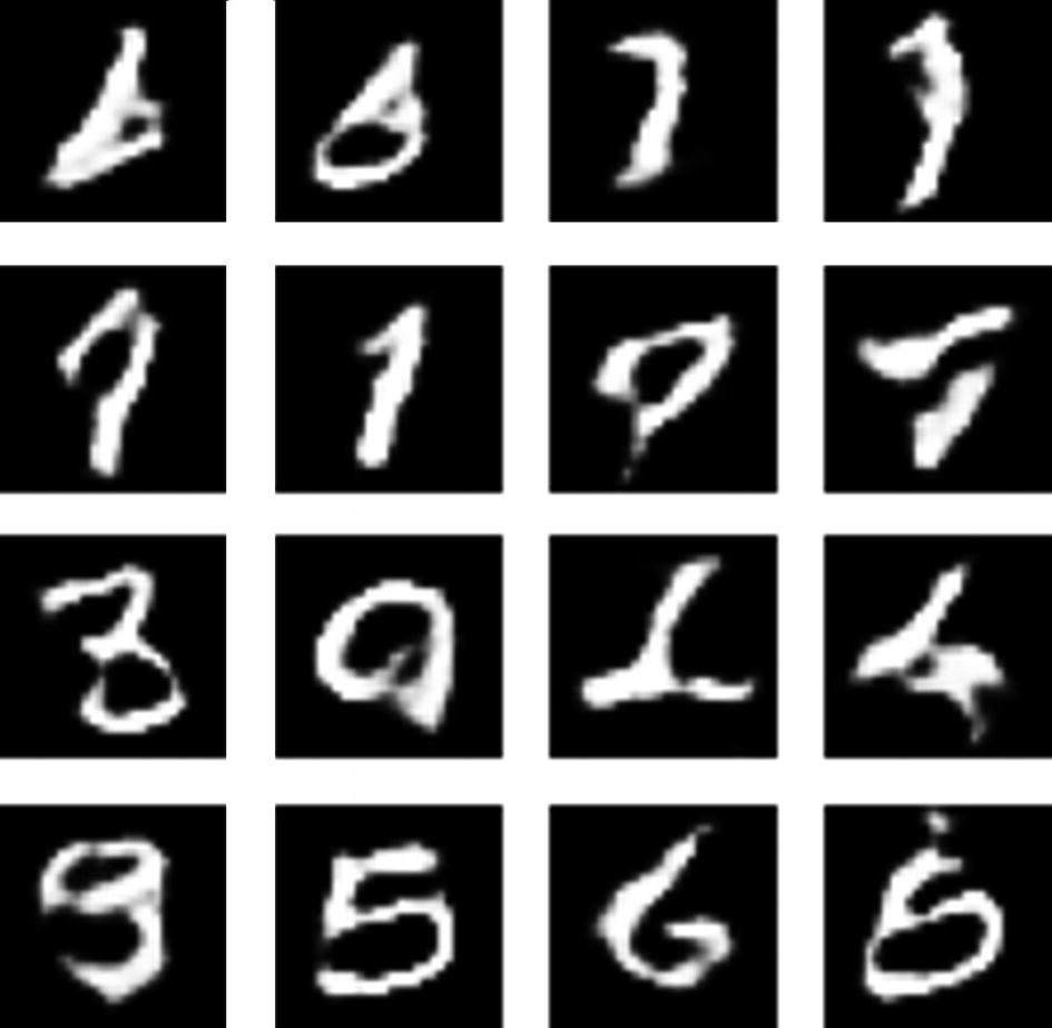
Starting the training loop is very easy. The single line of the following code would start training with the train function, which loops over the train_step() function and generates images using generate_and_save_images() function. We also receive stats and info during the process, as well as the generated images on a 4 x 4 grid layout.

train(train_dataset, EPOCHS)

Output:

Figure 12-5

The Generated Images After 60 Epochs in 4 x 4 Grid Layout

As you can see in Figure 12-5, after 60 epochs, the generated images are very close to proper handwritten digits. The only digit I cannot spot is the digit two (2), which could just be a coincidence.

Now that we trained our model and saved our checkpoints, we can restore the trained model with the following line:

checkpoint.restore(tf.train.latest_checkpoint(checkpoint_dir))

Animate Generated Digits During the Training

During the training, our generate_and_save_images() function successfully saved a 4 x 4 generated image grid layout at each epoch. Let’s see how our model’s generative abilities evolve over time with a simple exercise.

To be able to open the images, we can use PIL (Python Image Library), which supports many different image formats, including PNG. We can define a custom function to open images with the following lines:

# PIL is a library which may open different image file formats

import PIL

# Display a single image using the epoch number

def display_image(epoch_no):

  return PIL.Image.open( 'image_at_epoch_{:04d}.png'.format( epoch_no ))

Now test the function with the following line, which would display the latest PNG file generated by our model:

display_image(EPOCHS)

Output is shown in Figure 12-6:

Figure 12-6

The Display of the Latest PNG File Generated by the GAN Model. Note That They Are Identical to Samples Shown in Figure 12-5. Since We Restored the Model from the Last Checkpoint

With display_images() function , we may display any image we want. On top of this option, wouldn’t it be cool to generate an animated GIF image showing how our model evolved over time? We can achieve this using glob and imageio libraries, which would pile up all the PNG files to create an animated GIF file. The following lines do this task:

import glob # The glob module is used for Unix style pathname pattern expansion.

import imageio # The library that provides an easy interface to read and write a wide range of image data

anim_file = 'dcgan.gif'

with imageio.get_writer(anim_file, mode="I") as writer:

  filenames = glob.glob('image*.png')

  filenames = sorted(filenames)

  for filename in filenames:

    image = imageio.imread(filename)

    writer.append_data(image)

  image = imageio.imread(filename)

  writer.append_data(image)

Click the Files icon on the left side of your Google Colab Notebook to view all the files, including ‘dcgan.gif’. You can simply download it to view an animated version of the images our model generated at each epoch. To be able to view the GIF image within your Google Colab Notebook, you can use the following line:

display.Image(open('dcgan.gif','rb').read())

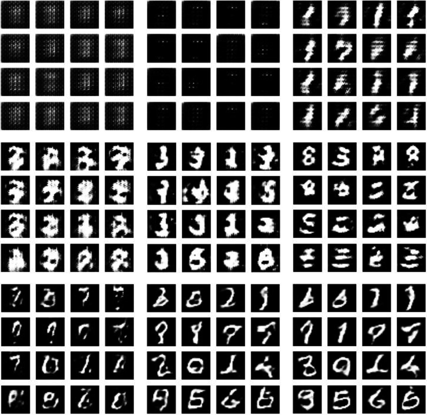
Figure 12-7 shows several frames from the GIF image we created:

Figure 12-7

Generated Digit Examples from the Different Epochs. See How the GAN Model Learns to Generate Digits Over Time

Conclusion

In this chapter, we covered our last neural network architecture, generative adversarial networks, which are mainly used for generative tasks in fields such as art, manufacturing, research, and gaming. We also conducted a case study, in which we trained a GAN model which is capable of generating handwritten digits.

Footnotes

1

Deep Convolutional Generative Adversarial Network, TensorFlow, available at www.tensorflow.org/tutorials/generative/dcgan