© Orhan Gazi Yalçın 2021

O. G. YalçınApplied Neural Networks with TensorFlow 2https://doi.org/10.1007/978-1-4842-6513-0_6

6. Feedforward Neural Networks

Orhan Gazi Yalçın¹  

(1)

Istanbul, Turkey

 

In this chapter, we will cover the most generic version of neural networks, feedforward neural networks. Feedforward neural networks are a group of artificial neural networks in which the connections between neurons do not form a cycle. Connections between neurons are unidirectional and move in only forward direction from input layer through hidden layers and to output later. In other words, the reason these networks are called feedforward is that the flow of information takes place in the forward direction.

Recurrent Neural Networks

which we will cover in Chapter 8, are improved versions of feedforward neural networks in which bidirectionality is added. Therefore, they are not considered feedforward anymore.

Feedforward neural networks are mainly used for supervised learning tasks. They are especially useful in analytical applications and quantitative studies where traditional machine learning algorithms are also used.

Feedforward neural networks are very easy to build, but they are not scalable in computer vision and natural language processing (NLP) problems. Also, feedforward neural networks do not have a memory structure which is useful in sequence data. To address the scalability and memory issues, alternative artificial neural networks such as convolutional neural networks and recurrent neural networks are developed, which will be covered in the next chapters.

You may run into different names for feedforward neural networks such as artificial neural networks, regular neural networks, regular nets, multilayer perceptron, and some others. There is unfortunately an ambiguity, but in this book, we always use the term feedforward neural network.

Deep and Shallow Feedforward Neural Networks

Every feedforward neural network must have two layers: (i) an input layer and (ii) an output layer. The main goal of a feedforward neural network is to approximate a function using (i) the input values fed from the input layer and (ii) the final output values in the output layer by comparing them with the label values.

Shallow Feedforward Neural Network

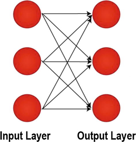
When a model only has an input and an output layer for function approximation, it is considered as a shallow feedforward neural network. It is also referred to as single-layer perceptron, shown in Figure 6-1.

Figure 6-1

Shallow Feedforward Neural Network or Single-Layer Perceptron

The output values in a shallow feedforward neural network are computed directly from the sum of the product of its weights with the corresponding input values and some bias. Shallow feedforward neural networks are not useful to approximate nonlinear functions. To address this issue, we embed hidden layers between input and output layers.

Deep Feedforward Neural Network

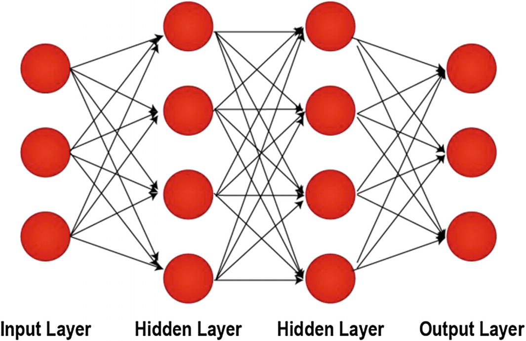
When a feedforward neural network has one or more hidden layers which enable it to approximate more complex function, this model is considered as a deep feedforward neural network. It is also referred to as multilayer perceptron, shown in Figure 6-2.

Figure 6-2

Deep Feedforward Neural Network or Multilayer Perceptron

Every neuron in a layer is connected to the neurons in the next layer and utilizes an activation function.

Universal Approximation Theory

indicates that a feedforward neural network can approximate any real-valued continuous functions on compact subsets of Euclidean space. The theory also implies that when given appropriate weights, neural networks can represent all the potential functions.

Since deep feedforward neural networks can approximate any linear or nonlinear function, they are widely used in real-world applications, both for classification and regression problems. In the case study of this chapter, we also build a deep feedforward neural network to have acceptable results.

Feedforward Neural Network Architecture

In a feedforward neural network, the leftmost layer is called the input layer, consisting of input neurons. The rightmost layer is called the output layer, consisting of a set of output neurons or a single output neuron. The layers in the middle are called hidden layers with several neurons ensuring nonlinear approximation.

In a feedforward neural network, we take advantage of an optimizer with backpropagation, activation functions, and cost functions as well as additional bias on top of weights. These terms are already explained in Chapter 3 and, therefore, omitted here. Please refer to Chapter 3 for more detail. Let’s take a deeper look at the layers of feedforward neural networks.

Layers in a Feedforward Neural Network

As mentioned earlier, our generic feedforward neural network architecture consists of three types of layers:

• An input layer

• An output layer

• A number of hidden layers

Input Layer

Input layer is the very first layer of feedforward neural network, which is used to feed data into the network. Input layer does not utilize an activation function and its sole purpose to get the data into the system. The number of neurons in an input layer must be equal to the number of features (i.e., explanatory variables) fed into the system. For instance, if we are using five different explanatory variables to predict one response variable, our model’s input layer must have five neurons.

Output Layer

Output layer is the very last layer of the feedforward neural network, which is used to output the prediction. The number of neurons in the output layer is decided based on the nature of the problem. For regression problems, we aim to predict a single value, and therefore, we set a single neuron in our output layer. For classification problems, the number of neurons is equal to the number of classes. For example, for binary classification, we need two neurons in the output layer, whereas for multi-class classification with five different classes, we need five neurons in the output layer. Output layers also take advantage of an activation function depending on the nature of the problem (e.g., a linear activation for regression and softmax for classification problems).

Hidden Layer

Hidden layers are created to ensure the approximation of the nonlinear functions. We can add as many hidden layers as we desire, and the number of neurons at each layer can be changed. Therefore, as opposed to input and output layers, we are much more flexible with hidden layers. Hidden layers are appropriate layers to introduce bias terms, which are not neurons, but constants added to the calculations that affect each neuron in the next layer. Hidden layers also take advantage of activation functions such as Sigmoid, Tanh, and ReLU.

In the next section, we will build a deep feedforward neural network to show all these layers in action. Thanks to Keras Sequential API, the process will be very easy.

Case Study | Fuel Economics with Auto MPG

Now that we covered the basics of feedforward neural networks, we can build a deep feedforward neural network to predict how many miles can a car travel with one gallon of gas. This term is usually referred to as miles per gallon (MPG). For this case study, we use one of the classic datasets: Auto MPG dataset. Auto MPG was initially used in the 1983 American Statistical Association Exposition. The data concerns prediction of city-cycle fuel consumption in miles per gallon in terms of three multivalued discrete and five continuous attributes. For this case study, we benefit from a tutorial written by François Chollet, the creator of Keras library.¹

Let’s dive into the code. Please create a new Colab Notebook via https://colab.research.google.com.

Initial Installs and Imports

We will take advantage of the TensorFlow Docs library which is not included in the Google Colab Notebook initially. So, we start the case study with a library installation with the following code:

# Install tensorflow_docs

!pip install -q git+https://github.com/tensorflow/docs

There are a number of libraries we will utilize in this case study. Let’s import the ones we will use in the beginning:

# Import the initial libraries to be used

import tensorflow as tf

import pandas as pd

import numpy as np

import matplotlib.pyplot as plt

Please note that there will be some other imports, which will be shared in their corresponding sections.

Downloading the Auto MPG Data

Even though Auto MPG is a very popular dataset, we still cannot access the dataset via TensorFlow’s dataset module. However, there is a very straightforward way (thanks to the get_file() function of tf.keras.utils module) to load external data into our Google Colab Notebook with the following lines of code:

autompg = tf.keras.utils.get_file(

        fname='auto-mpg', #filename for local directory

        origin='http://archive.ics.uci.edu/ml/machine-learning-databases/auto-mpg/auto-mpg.data',#URL address to retrieve the dataset

Note that we retrieve the dataset from UCI Machine Learning Repository. UC Irvine provides an essential repository, along with Kaggle, in which you can access to a vast number of popular datasets.

Data Preparation

When we look at the UC Irvine’s Auto MPG page, we can see a list of attributes which represents all the variables in the Auto MPG dataset, which is shared here:

Attribute Information:

• mpg: Continuous (response variable)

• cylinders: Multivalued discrete

• displacement: Continuous

• horsepower: Continuous

• weight: Continuous

• acceleration: Continuous

• model year: Multivalued discrete

• origin: Multivalued discrete

• car name: String (unique for each instance)

DataFrame Creation

As a best practice, we will name our dataset columns with these attribute names and import from our Google Colab directory since we already saved it in the previous section:

column_names = ['mpg', 'cylinders', 'displacement', 'HP', 'weight', 'acceleration', 'modelyear', 'origin']

df = pd.read_csv(autompg, # name of the csv file

        sep=" ", # separator in the csv file

        comment='\t', #remove car name sep. with '\t'

        names=column_names,

        na_values = '?', #NA values are coded as '?'

        skipinitialspace=True)

df.head(2) #list the first two row of the dataset

Here is the result of df.head(2), shown in Figure 6-3.

Figure 6-3

The First Two Lines of the Auto MPG Dataset

Dropping Null Values

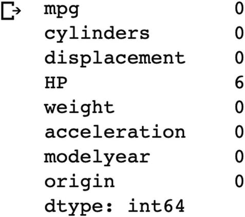
We can check the number of null values with the following code:

df.isna().sum()

The output we get is shown in Figure 6-4.

Figure 6-4

Null Value Counts in the Auto MPG Dataset

We have six null values in the HP column. There are several ways to deal with the null values. Firstly, we can drop them. Secondly, we can fill them using a method such as (a) filling with the mean value of other observations or (b) use a regression method to interpolate their value. For the sake of simplicity, we will drop them with the following code:

df = df.dropna() # Drop null values

df = df.reset_index(drop=True) # Reset index to tidy up the dataset

df.show()

Handling Categorical Variables

Let’s review our dataset with the info attribute of Pandas DataFrame object:

df.info() # Get an overview of the dataset

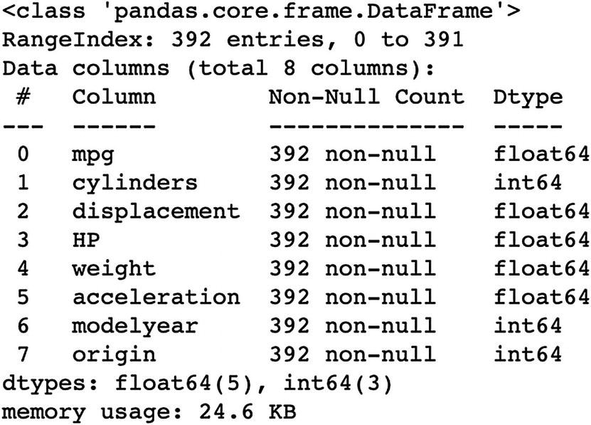
As shown in Figure 6-5, We can see that Auto MPG dataset has 392 car observations with no null values. The variables cylinders, modelyear, and origin are the categorical variables we should consider using dummy variables.

Figure 6-5

Overview of the Auto MPG Dataset

Dummy Variable

is a special variable type that takes only the value 0 or 1 to indicate the absence or presence of a categorical effect. In machine learning studies, every category of a categorical variable is encoded as a dummy variable. But, omitting one of these categories as a dummy variable is a good practice, which prevents multicollinearity problem.

Using dummy variables is especially important if the values of a categorical variable do not indicate a mathematical relationship. This is absolutely valid for origin variable since the values 1, 2, and 3 represent the United States, Europe, and Japan. Therefore, we need to generate dummies for origin variable, drop the first one to prevent multicollinearity, and drop the initial origin variable (origin variable is now represented with the generated dummy variables). We can achieve these tasks with the following lines of code:

def one_hot_origin_encoder(df):

        df_copy = df.copy()

        df_copy['EU']=df_copy['origin'].map({1:0,2:1,3:0})

        df_copy['Japan']=df_copy['origin'].map({1:0,2:0,3:1})

        df_copy = df_copy.drop('origin',axis=1)

        return df_copy

df_clean = one_hot_origin_encoder(df)

Here is the result of df_clean.head(2), shown in Figure 6-6.

Figure 6-6

The First Two Lines of the Auto MPG Dataset with Dummy Variables

Splitting Auto MPG for Training and Testing

Now that we cleaned our dataset, it is time to split them into train and test sets. Train set is used to train our neural network (i.e., optimize the neuron weights) to minimize the errors. Test set is used as the never-been-seen observations to test the performance of our trained neural network.

Since our dataset is in the form of a Pandas DataFrame object, we can use sample attribute. We keep the 80% of the observations for training and 20% for testing. Additionally, we also split the label from the features so that we can feed the features as input. Then, check the results with labels.

These tasks can be achieved with the following lines of codes:

# Training Dataset and X&Y Split

# Test Dataset and X&Y Split

# For Training

train = df_clean.sample(frac=0.8,random_state=0)

train_x = train.drop('mpg',axis=1)

train_y = train['mpg']

# For Testing

test = df_clean.drop(train.index)

test_x = test.drop('mpg',axis=1)

test_y = test['mpg']

Now that we split our dataset into train and test sets, it is time to normalize our data. As mentioned in Chapter 3, feature scaling is an important part of the data preparation. Without feature scaling, a feature can adversely affect our model.

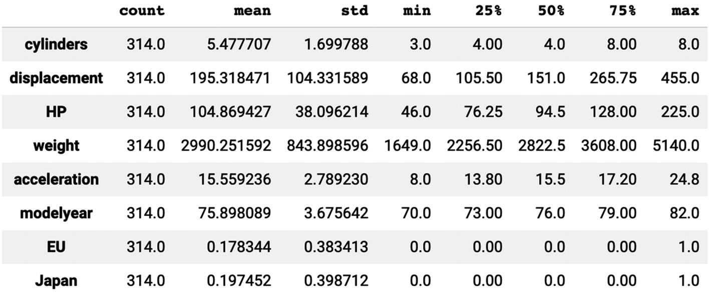
We need to extract the means and standard deviations to manually apply normalization to our data. We can generate this dataset with ease, using the following code:

train_stats = train_x.describe().transpose()

You can obtain the following output in Figure 6-7 by running train_stats.

Figure 6-7

train_stats DataFrame for Train Set Statistics

Now that we have the mean and standard deviation values for training set features, it is time to normalize the train and test sets. The custom normalizer(x) function can be used for train, test, and new observation sets.

# Feature scaling with the mean

# and std. dev. values in train_stats

def normalizer(x):

  return (x-train_stats['mean'])/train_stats['std']

train_x_scaled = normalizer(train_x)

test_x_scaled = normalizer(test_x)

Note that we do not normalize the label (y) values since their wide range doesn’t pose a threat for our model.

Model Building and Training

Now, our data is cleaned and prepared for our feedforward neural network pipeline. Let’s build our model and train it.

Tensorflow Imports

We already had some initial imports. In this part, we will import the remaining modules and libraries to build, train, and evaluate our feedforward neural network.

Remaining imports consist of the following libraries:

# Importing the required Keras modules containing model and layers

from tensorflow.keras.models import Sequential

from tensorflow.keras.layers import Dense

# TensorFlow Docs Imports for Evaluation

import tensorflow_docs as tfdocs

import tensorflow_docs.plots

import tensorflow_docs.modeling

Sequential() is our API for model building, whereas Dense() is the layer we will use in our feedforward neural network. tf.docs module will be used for model evaluation.

Model with Sequential API

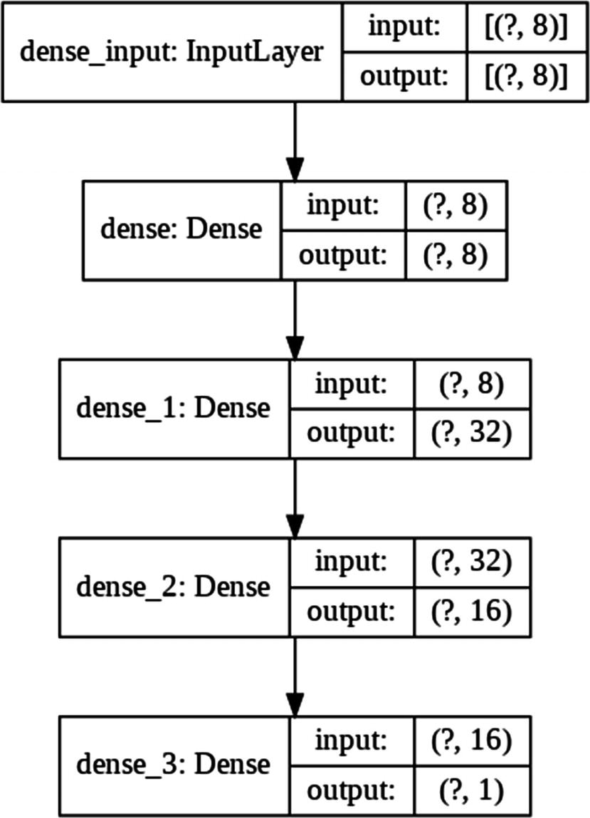
After creating a model object with Sequential API and naming it model, we can shape our empty model by adding Dense() layers. Each dense layer – except the last one – requires an activation function. We will use ReLU for this case study, but feel free to set other activation functions such as Tanh or Sigmoid. Our input_shape parameter must be equal to the number of features, and our output layer must have only one neuron since this is a regression case.

# Creating a Sequential Model and adding the layers

model = Sequential()

model.add(Dense(8,activation=tf.nn.relu, input_shape= [train_x.shape[1]])),

model.add(Dense(32,activation=tf.nn.relu)),

model.add(Dense(16,activation=tf.nn.relu)),

model.add(Dense(1))

We can see the flowchart of model with a single line of code; see Figure 6-8:

tf.keras.utils.plot_model(model, show_shapes=True)

Figure 6-8

The Flowchart of the Feedforward Neural Network for Auto MPG

Model Configuration

Now that we build the main network structure of our neural network, we need to configure our optimizer, cost function, and metrics before initiating the training. We will use Adam optimizer and mean squared error (MSE) in our neural network. Additionally, TensorFlow will provide us mean absolute error (MAE) values as well as MSE values. We can configure our model with the following code:

# Optimizer, Cost, and Metric Configuration

model.compile(optimizer='adam',

              loss='mse',

              metrics=['mse','mae']

)

As mentioned in Chapter 3, one of the powerful methods to fight overfitting is early stopping. With the following lines of code, we will set an early stopper if we do not see a valuable improvement for 50 epochs.

# Early Stop Configuration

early_stop=tf.keras.callbacks.EarlyStopping( monitor="val_loss", patience=50)

Now that we configured our model, we can train our model with the fit attribute of our model object:

# Fitting the Model and Saving the Callback Histories

history=model.fit(

        x=train_x_scaled,

        y=train_y,

        epochs=1000,

        validation_split = 0.2,

        verbose=0,

        callbacks=[early_stop,

                tfdocs.modeling.EpochDots()

                ])

We set aside 20% of our train set for validation. Therefore, our neural network will evaluate the model even before the test set. We set the epoch value to 1000, but it will stop early if it cannot observe a valuable improvement on the validation loss/cost. Finally, callbacks parameter will save valuable information for us to evaluate our model with plots and other useful tools.

Evaluating the Results

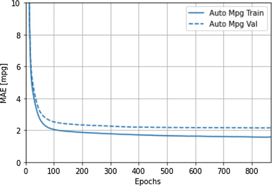
Now that we trained our model, we can evaluate the results. Our TensorFlow Docs library allows us to plot the loss values at each epoch. We can create a new object using HistoryPlotter to create the object with following code:

plot_obj=tfdocs.plots.HistoryPlotter(smoothing_std=2)

After creating the object, we can use the plot attribute to create the plot, and we can set the ylim and ylabel values just as in Matplotlib with the following code:

plot_obj.plot({'Auto MPG': history}, metric = "mae")

plt.ylim([0, 10])

plt.ylabel('MAE [mpg]')

Figure 6-9 shows the overview of our loss values at each epoch.

Figure 6-9

The Line Plot Showing Mean Absolute Error Values at Each Epoch

With the evaluate attribute of the model, we can also evaluate our model using test set. The following lines will generate loss, MAE, and MSE values using our test set as shown in Figure 6-10:

loss,mae,mse=model.evaluate(test_x_scaled,

                            test_y,

                            verbose=2)

print("Testing set Mean Abs Error: {:5.2f} MPG".format(mae))

Figure 6-10

Evaluation Results for the Trained Model for Auto MPG

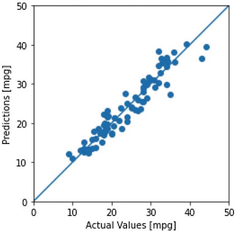
We can generate predictions using the test set labels with a single line of code:

test_preds = model.predict(test_x_scaled).flatten()

Finally, we can plot the test set labels (actual values) against the predictions generated with the test set features (see Figure 6-11) with the following lines of code:

evaluation_plot = plt.axes(aspect='equal')

plt.scatter(test_y, test_preds)#Scatter Plot

plt.ylabel('Predictions [mpg]')#Y for Predictions

plt.xlabel('Actual Values [mpg]')#X for Actual Values

plt.xlim([0, 50])

plt.ylim([0, 50])

plt.plot([0, 50], [0, 50]) #line plot for comparison

Figure 6-11

The Scatter Plot for Actual Test Labels vs. Their Prediction Values

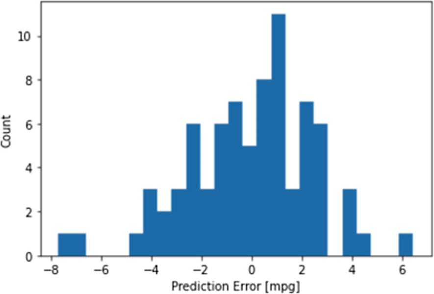
We can also generate a histogram showing the distribution of error terms around zero (see Figure 6-12), which is an important indication of bias in our model. The following lines of code generate the said histogram:

error = test_preds - test_y

plt.hist(error, bins = 25)

plt.xlabel("Prediction Error [mpg]")

plt.ylabel("Count")

Figure 6-12

The Histogram Showing the Error Distribution of the Model Around Zero

Making Predictions with a New Observation

Both the scatter plot and the histogram we generated earlier show that our model is healthy, and our loss values are also in an acceptable range. Therefore, we can use our trained model to make new predictions, using our own dummy observation.

I will create a dummy car with the following lines of code:

# Prediction for Single Observation

# What is the MPG of a car with the following info:

new_car = pd.DataFrame([[8,  #cylinders

                         307.0, #displacement

                         130.0, #HP

                         5504.0, #weight

                         12.0, #acceleration

                         70, #modelyear

                         1 #origin

          ]], columns=column_names[1:])

This code will create the following Pandas DataFrame with single observation, shown in Figure 6-13.

Figure 6-13

A Pandas DataFrame with Single Observation

We need to create dummy variables and normalize the observation before feeding into the trained model. After these operations, we can simply use the predict attribute of our model. We can complete these operations with these lines:

new_car = normalizer(one_hot_origin_encoder(new_car))

new_car_mpg = model.predict(new_car).flatten()

print('The predicted miles per gallon value for this car is:', new_car_mpg)

The preceding code gives this output:

The prediction miles per gallon value for this car is: [14.727904]

Conclusion

Feedforward neural networks are artificial neural networks that are widely used in analytical applications and quantitative studies. They are the oldest artificial neural networks and often named as multilayer perceptron. They are considered as the backbone of the artificial neural network family. You can find them embedded at the end of a convolutional neural network. Recurrent neural networks are developed from feedforward neural networks, with added bidirectionality.

In the next chapter, we will dive into convolutional neural networks, a group of neural network family which are widely used in computer vision, image and video processing, and many alike.

Footnotes

1

Copyright (c) 2017 François Chollet

Permission is hereby granted, free of charge, to any person obtaining a copy of this software and associated documentation files (the “Software”), to deal in the Software without restriction, including without limitation the rights to use, copy, modify, merge, publish, distribute, sublicense, and/or sell copies of the Software, and to permit persons to whom the Software is furnished to do so, subject to the following conditions:

The above copyright notice and this permission notice shall be included in all copies or substantial portions of the Software.

THE SOFTWARE IS PROVIDED “AS IS”, WITHOUT WARRANTY OF ANY KIND, EXPRESS OR IMPLIED, INCLUDING BUT NOT LIMITED TO THE WARRANTIES OF MERCHANTABILITY, FITNESS FOR A PARTICULAR PURPOSE AND NONINFRINGEMENT. IN NO EVENT SHALL THE AUTHORS OR COPYRIGHT HOLDERS BE LIABLE FOR ANY CLAIM, DAMAGES OR OTHER LIABILITY, WHETHER IN AN ACTION OF CONTRACT, TORT OR OTHERWISE, ARISING FROM, OUT OF OR IN CONNECTION WITH THE SOFTWARE OR THE USE OR OTHER DEALINGS IN THE SOFTWARE.