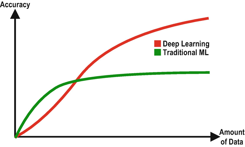
Deep Learning vs. Traditional ML Comparison on Accuracy
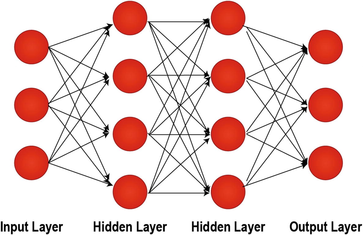
A Depiction of Artificial Neural Networks with Two Hidden Layers
You might think that deep learning is a newly invented field that recently overthrown the other machine learning algorithms. Lots of people think this way. However, the field of artificial neural networks and deep learning dates back to the 1940s. The recent rise of deep learning is mainly due to a high amount of available data and – more importantly – due to cheap and abundant processing power.
This is an overview chapter for deep learning. We will take a look at the critical concepts that we often use in deep learning, including (i) activation functions, (ii) loss functions, (iii) optimizers and backpropagation, (iv) regularization, and (v) feature scaling. But, first, we will dive into the history of artificial neural networks and deep learning so that you will have an idea about the roots of the deep learning concepts which you will often see in this book.
Timeline of Neural Networks and Deep Learning Studies
The timeline of neural networks and deep learning studies does not consist of a series of uninterrupted advancements. In fact, the field of artificial intelligence experienced a few downfalls, which are referred to as AI winters. Let’s dive into the history of neural networks and deep learning, which started in 1943.
Development of Artificial Neurons – In 1943, the pioneer academics Walter Pitts and Warren McCulloch published the paper “A Logical Calculus of the Ideas Immanent in Nervous Activity,” where they presented a mathematical model of a biological neuron, called McCulloch-Pitts Neuron . Capabilities of McCulloch Pitts Neuron are minimal, and it does not have a learning mechanism. The importance of McCulloch Pitts Neuron is that it lays the foundation for deep learning. In 1957, Frank Rosenblatt published another paper, titled “The Perceptron: A Perceiving and Recognizing Automaton,” where he introduces the perceptron with learning and binary classification capabilities. The revolutionary perceptron model – risen to its place after Mcculloch Pitts Neuron – has inspired many researchers working on artificial neural networks.
Backpropagation – In 1960, Henry J. Kelley published a paper titled “Gradient Theory of Optimal Flight Paths,” where he demonstrates an example of continuous backpropagation. Backpropagation is an important deep learning concept that we will cover under this chapter. In 1962, Stuart Dreyfus improved backpropagation with chain rule in his paper, “The Numerical Solution of Variational Problems.” The term backpropagation was coined in 1986 by Rumelhart, Hinton, and Williams, and these researchers have popularized its use in artificial neural networks.
Training and Computerization – In 1965, Alexey Ivakhnenko, usually referred to as “Father of Deep Learning,” built a hierarchical representation of neural networks and successfully trained this model by using a polynomial activation function. In 1970, Seppo Linnainmaa found automatic differentiation for backpropagation and was able to write the first backpropagation program. This development may be marked as the beginning of the computerization of deep learning. In 1971, Ivakhnenko created an eight-layer neural network, which is considered a deep learning network due to its multilayer structure.
AI Winter – In 1969, Marvin Minsky and Seymour Papert wrote the book Perceptrons in which he fiercely attacks the work of Frank Rosenblatt, the Perceptron. This book caused devastating damage to AI project funds, which triggered an AI winter that lasted from 1974 until 1980.
Convolutional Neural Networks – In 1980, Kunihiko Fukushima introduced the neocognitron, the first convolutional neural networks (CNNs), which can recognize visual patterns. In 1982, Paul Werbos proposed the use of backpropagation in neural networks for error minimization, and the AI community has adopted this proposal widely. In 1989, Yann LeCun used backpropagation to train CNNs to recognize handwritten digits in the MNIST (Modified National Institute of Standards and Technology) dataset. In this book, we have a similar case study in Chapter 7.
Recurrent Neural Networks – In 1982, John Hopfield introduced Hopfield network, which is an early implementation of recurrent neural networks (RNNs). Recurrent neural networks are revolutionary algorithms that work best for sequential data. In 1985, Geoffrey Hinton, David H. Ackley, and Terrence Sejnowski proposed Boltzmann Machine, which is a stochastic RNN without an output layer. In 1986, Paul Smolensky developed a new variation of Boltzmann Machine, which does not have intralayer connections in input and hidden layers, which is called a Restricted Boltzmann Machine. Restricted Boltzmann Machines are particularly successful in recommender systems. In 1997, Sepp Hochreiter and Jürgen Schmidhuber published a paper on an improved RNN model, long short-term memory (LSTM), which we will also cover in Chapter 8. In 2006, Geoffrey Hinton, Simon Osindero, and Yee Whye Teh combined several Restricted Boltzmann Machines (RBMs) and created deep belief networks, which improved the capabilities of RBMs.
Capabilities of Deep Learning – In 1986, Terry Sejnowski developed NETtalk, a neural network-based text-to-speech system which can pronounce English text. In 1989, George Cybenko showed in his paper “Approximation by Superpositions of a Sigmoidal Function” that a feedforward neural network with a single hidden layer can solve any continuous function.
Vanishing Gradient Problem – In 1991, Sepp Hochreiter discovered and proved the vanishing gradient problem, which slows down the deep learning process and makes it impractical. After 20 years, in 2011, Yoshua Bengio, Antoine Bordes, and Xavier Glorot showed that using Rectified Linear Unit (ReLU) as the activation function can prevent vanishing gradient problem.
GPU for Deep Learning – In 2009, Andrew Ng, Rajat Raina, and Anand Madhavan, with their paper “Large-Scale Deep Unsupervised Learning Using Graphics Processors,” recommended the use of GPUs for deep learning since the number of cores found in GPUs is a lot more than the ones in CPUs. This switch reduces the training time of neural networks and makes their applications more feasible. Increasing use of GPUs for deep learning has led to the development of specialized ASICS for deep learning (e.g., Google’s TPU) along with official parallel computing platforms introduced by GPU manufacturers (e.g., Nvidia’s CUDA and AMD’s ROCm).
ImageNet and AlexNet – In 2009, Fei-Fei Li launched a database with 14 million labeled images, called ImageNet. The creation of the ImageNet database has contributed to the development of neural networks for image processing since one of the essential components of deep learning is abundant data. Ever since the creation of the ImageNet database, yearly competitions were held to improve the image processing studies. In 2012, Alex Krizhevsky designed a GPU-trained CNN, AlexNet, which increased the model accuracy by 75% compared to earlier models.
Generative Adversarial Networks – In 2014, Ian Goodfellow came up with the idea of a new neural network model while he was talking with his friends at a local bar. This revolutionary model, which was designed overnight, is now known as generative adversarial neural networks (GANs), which is capable of generating art, text, and poems, and it can complete many other creative tasks. We have a case study for the implementation of GANs in Chapter 12.
Power of Reinforcement Learning – In 2016, DeepMind trained a deep reinforcement learning model, AlphaGo, which can play the game of Go, which is considered a much more complicated game compared to Chess. AlphaGo beat the World Champion Ke Jie in Go in 2017.
Turing Award to the Pioneers of Deep Learning – In 2019, the three pioneers in AI, Yann LeCun, Geoffrey Hinton, and Yoshua Bengio, shared the Turing Award. This award is proof that shows the significance of deep learning for the computer science community.
Structure of Artificial Neural Networks
Before diving into essential deep learning concepts, let’s take a look at the journey on the development of today’s modern deep neural networks. Today, we can easily find examples of neural networks with hundreds of layers and thousands of neurons, but before the mid twentieth century, the term artificial neural network did not even exist. It all started in 1943 with a simple artificial neuron – McCulloch Pitts Neuron – which can only do simple mathematical calculations with no learning capability.
McCulloch-Pitts Neuron
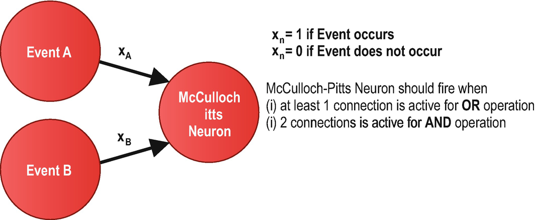
McCulloch Pitts Neuron for OR and AND Operations
Since the inputs from the events in McCulloch Pitts Neuron can only be Boolean values (0 or 1), its capabilities were minimal. This limitation was addressed with the development of Linear Threshold Unit (LTU).
Linear Threshold Unit (LTU)

Linear Threshold Unit (LTU) Visualization
Perceptron
Perceptron is a binary classification algorithm for supervised learning and consists of a layer of LTUs. In a perceptron, LTUs use the same event outputs as input. The perceptron algorithm can adjust the weights to correct the behavior of the trained neural network. In addition, a bias term may be added to increase the accuracy performance of the network.

An Example of a Single-Layer Perceptron Diagram
A Modern Deep Neural Network
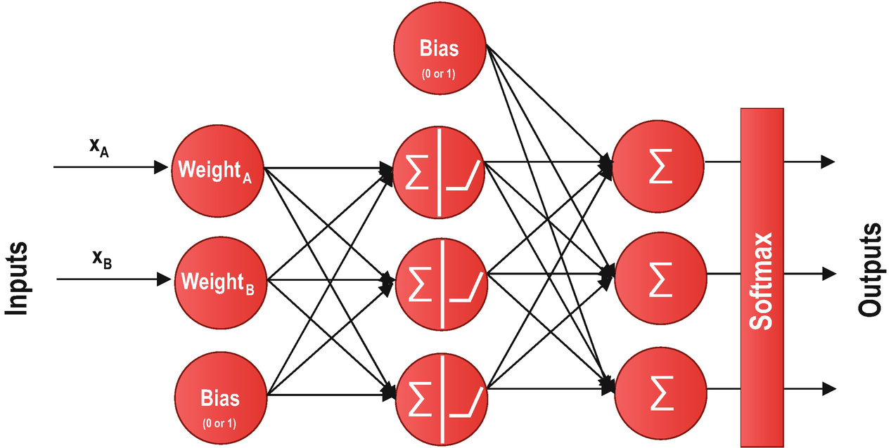
A Modern Deep Neural Network Example
Now that you know more about the journey to develop today’s modern deep neural networks, which started with the McCulloch Pitts Neurons, we can dive into essential deep learning concepts that we use in our applications.
Activation Functions
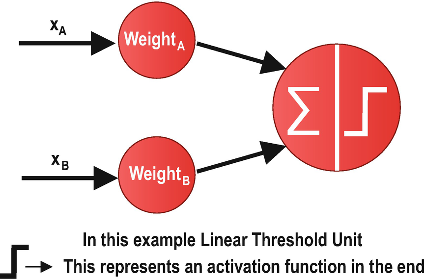
An Example LTU Diagram with Activation Function in the End
Activation functions introduce a final calculation step that adds additional complexity to artificial neural networks. Therefore, they increase the required training time and processing power. So, why would we use activation functions in neural networks? The answer is simple: Activation functions increase the capabilities of the neural networks to use relevant information and suppress the irrelevant data points. Without activation functions, our neural networks would only be performing a linear transformation. Although avoiding activation functions makes a neural network model simpler, the model will be less powerful and will not be able to converge on complex pattern structures. A neural network without an activation function is essentially just a linear regression model.
Binary Step
Linear
Sigmoid (Logistic Activation Function)
Tanh (Hyperbolic Tangent)
ReLU (Rectified Linear Unit)
Softmax
Leaky ReLU
Parameterized ReLU
Exponential Linear Unit
Swish

Plots for Tanh, ReLU, and Sigmoid Functions
ReLU function is a widely used general-purpose activation function. It should be used in hidden layers. In case there are dead neurons, Leaky ReLU may fix potential problems.
The Sigmoid function works best in classification tasks.
Sigmoid and Tanh functions may cause vanishing gradient problem.
The best strategy for an optimized training practice is to start with ReLU and try the other activation functions to see if the performance improves .
Loss (Cost or Error) Functions

Error = Measured Value - Predicted Value
Therefore, we end up with an error term for each prediction we make. Imagine you are working with millions of data points. To be able to derive insights from these individual error terms, we need an aggregative function so that we can come up with a single value for performance evaluation. This function is referred to as loss function, cost function , or error function , depending on the context.
Several loss functions are used for performance evaluation, and choosing the right function is an integral part of model building. This selection must be based on the nature of the problem. While Root Mean Squared Error (RMSE) function is the right loss function for regression problems in which we would like to penalize large errors, multi-class crossentropy should be selected for multi-class classification problems.
In addition, to be used to generate a single value for aggregated error terms, the loss function may also be used for rewards in reinforcement learning. In this book, we will mostly use loss functions with error terms, but beware that it is possible to use loss functions as a reward measure.
Several loss functions are used in deep learning tasks. Root mean squared error (RMSE), mean squared error (MSE), mean absolute error (MAE), and mean absolute percentage error (MAPE) are some of the appropriate loss functions for regression problems. For binary and multi-class classification problems, we can use variations of crossentropy (i.e., logarithmic) function .
Optimization in Deep Learning

Deep Learning Model Training with Cost Function, Activation Function, and Optimizer
There are several optimization algorithms and challenges encountered during the optimization process. In this section, we will briefly introduce these functions and challenges. But first, let’s take a look at an essential optimization concept: backpropagation.
Backpropagation
Step 1: The trained neural network makes a prediction with the current weights and biases.
Step 2: The performance of the neural network is measured with a loss function as a single error measure.
Step 3: This error measure is backpropagated to optimizer so that it can readjust the weights and biases.
Repeat
By using the information provided by the backpropagation algorithm , optimization algorithms can perfect the weights and biases used in the neural network. Let’s take a look at the optimization algorithms (i.e., optimizers), which are used in parallel with the backpropagation mechanism.
Optimization Algorithms
Adam
Stochastic gradient descent (SGD)
Adadelta
Rmsprop
Adamax
Adagrad
Nadam
Note that all of these optimizers are readily available in TensorFlow as well as the loss and activation functions, which are previously mentioned . The most common ones used in real applications are Adam optimizer and Stochastic gradient descent (SGD) optimizer. Let’s take a look at the mother of all optimizers, gradient descent and SGD, to have a better understanding of how an optimization algorithm works.
Gradient Descent and Stochastic Gradient Descent (SGD) – Stochastic gradient descent is a variation of gradient descent methods. SGD is widely used as an iterative optimization method in deep learning. The roots of SGD date back to the 1950s, and it is one of the oldest – yet successful – optimization algorithms.
Gradient descent methods are a family of optimization algorithms used to minimize the total loss (or cost) in the neural networks. There are several gradient descent implementations: The original gradient descent – or batch gradient descent – algorithm uses the whole training data per epoch. Stochastic (Random) gradient descent (SGD) selects a random observation to measure the changes in total loss (or cost) as a result of the changes in weights and biases. Finally, mini-batch gradient descent uses a small batch so that training may still be fast as well as reliable .
is the hyperparameter that represents the number of times that the values of a neural network are to be adjusted using the training dataset.

A Weight-Loss Plot Showing Gradient Descent
Figure 3-10 shows how gradient descent algorithm works. Larger incremental steps are taken when the machine learning expert selects a faster learning rate.
is the parameter in optimization algorithms which regulates the step size taken at each iteration while moving forward a minimum of a loss/cost function. With a fast learning rate, the model converges around the minimum faster, yet it may overshoot the actual minimum point. With a slow learning rate, optimization may take too much time. Therefore, a machine learning expert must choose the optimal learning rate, which allows the model to find the desired minimum point in a reasonable time.
Adam Optimizer – What Is Adam?
I will not dive into the details of the other optimization algorithms since they are mostly altered or improved implementations of gradient descent methods. Therefore, understanding the gradient descent algorithm will be enough for the time being .
In the next section, we see the optimization challenges which negatively affect the optimization process during training. Some of the optimization algorithms, as mentioned earlier, were developed to mitigate these challenges.
Optimization Challenges
There are three optimization challenges we often encounter in deep learning. These challenges are (i) local minima, (ii) saddle points, and (iii) vanishing gradients. Let’s briefly discuss what they are.
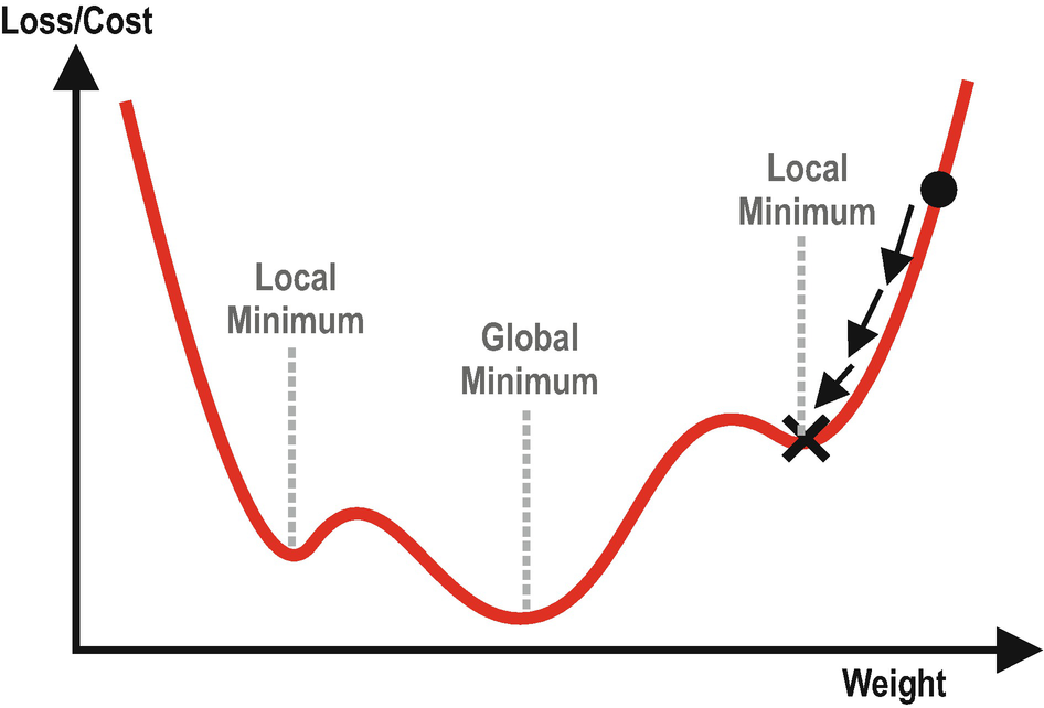
A Weight-Loss Plot with Two Local Minima and a Global Minimum
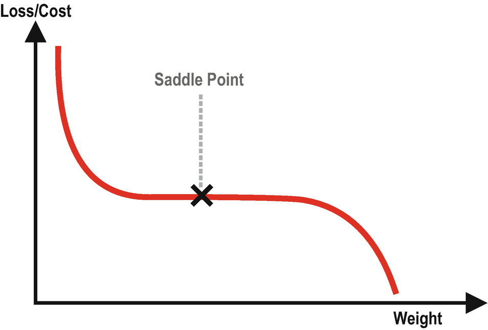
A Weight-Loss Plot with Two Local Minima and a Global Minimum

The Sigmoid Function and Its Derivative
To be able to solve this common optimization challenges , we should try and find the best combination of activation functions and optimization functions so that our model correctly converges and finds an ideal minimum point.
Overfitting and Regularization
Another important concept in deep learning and machine learning is overfitting. In this section, we cover the overfitting problem and how to address overfitting with regularization methods.
Overfitting

Underfitting and Overfitting in X-Y Plot
The solution to the underfitting problem is building a good model with meaningful features, feeding enough data, and training enough. On the other hand, more data, removing excessive features, and cross-validation are proper methods to fight the overfitting problem. In addition, we have a group of sophisticated methods to overcome overfitting problems, namely, regularization methods.
Regularization
Early stopping
Dropout
L1 and L2 regularization
Data augmentation
Early Stopping – Early stopping is a very simple – yet effective – strategy to prevent overfitting. Setting a sufficient number of epochs (training steps) is crucial to achieving a good level of accuracy. However, you may easily go overboard and train your model to fit too tightly to your training data. With early stopping, the learning algorithm is stopped if the model does not show a significant performance improvement for a certain number of epochs.
Dropout – Dropout is another simple – yet effective – regularization method. With dropout enabled, our model temporarily removes some of the neurons or layers from the network, which adds additional noise to the neural network. This noise prevents the model from fitting to the training data too closely and makes the model more flexible.
L1 and L2 Regularization – These two methods add an additional penalty term to the loss function, which penalizes the errors even more. For L1 regularization, this term is a lasso regression, whereas it is ridge regression for L2 regularization. L1 and L2 regularizations are particularly helpful when dealing with a large set of features.
Data Augmentation – Data augmentation is a method to increase the amount of training data. By making small transformations on the existing data, we can generate more observations and add them to the original dataset. Data augmentation increases the total amount of training data, which helps preventing the overfitting problem.
Feature Scaling
Standardization: It adjusts the values of each feature to have zero mean and unit variance.
Min-Max Normalization (Rescaling): It scales the values of each feature between [0, 1] and [-1, 1].
Mean Normalization: It deducts the mean from each data point and divides the result to max-min differential. It is a slightly altered and less popular version of min-max normalization.
Scaling to Unit Length: It divides each component of a feature by the Euclidian length of the vector of this feature.
It ensures that each feature contributes to the prediction algorithm proportionately.
It speeds up the convergence of the gradient descent algorithm, which reduces the time required for training a model.
Final Evaluations
In this chapter, we covered the timeline of artificial neural networks and deep learning. It helped us to understand how the concepts we use in our professional lives came to life after many years of research. The good news is that thanks to TensorFlow, we are able to add these components in our neural networks in a matter of seconds.
Following the deep learning timeline, we analyzed the structure of neural networks and the artificial neurons in detail. Also, we covered the fundamental deep learning concepts, including (i) optimization functions, (ii) activation functions, (iii) loss functions, (iv) overfitting and regularization, and (v) feature scaling.
This chapter serves as a continuation of the previous chapter where we cover the machine learning basics. In the next chapter, we learn about the most popular complementary technologies used in deep learning studies: (i) NumPy, (ii) SciPy, (iii) Matplotlib, (iii) Pandas, (iv) scikit-learn, and (v) Flask.