Designing the Study

Suppose you settled on a strategy for measuring love. Now you face another tough decision: how to design your data collection. Research on intimate relationships uses several study designs, each of which is appropriate for investigating different kinds of questions.

Correlational Research

Researchers conduct correlational research to study naturally occurring associations among variables; it is aimed primarily at answering descriptive questions. For example, are more intelligent people more satisfied with their intimate relationships? Are people whose parents divorced at higher risk of getting divorced themselves? Are couples happier when they share similar interests? Each of these questions asks how differences in one variable may be associated with differences in another variable. Measuring variables and describing their possible associations are relatively straightforward processes, and because many important questions about intimate relationships revolve around description, correlational studies account for much of this research. Virtually all studies describing gender differences are correlational—they examine how some variables may naturally differ among men and among women. Studies of cultural differences in relationships are also correlational—they describe how relationships may vary across cultures, localities, or ethnicities.

Pros and Cons When the goal is to examine how two or more variables are associated, no research design is more appropriate than a correlational study. Correlational research is also valuable for studying variables that cannot be manipulated or studied in other ways. Research on intimate relationships, for example, has explored how relationships are affected by a particular experience, such as a chronic illness, a previous bad relationship, or one partner’s affair. Obviously, researchers cannot create or control these experiences. But one way to study them is to divide couples into those who have or have not experienced these events and then study how other aspects of the relationship vary naturally across the groups.

For example, after Hurricane Hugo devastated parts of South Carolina in 1989, psychologists Catherine Cohan and Steve Cole (2002) wanted to know how the stress of coping with the disaster affected marriages in that part of the country. They could not change whether people experienced the event, but they could compare marriage and divorce rates in the counties that were struck by the hurricane to rates in similar nearby counties that were passed over. They found that divorce rates went up in counties affected by the hurricane, but so did marriage rates, suggesting that the crisis prompted couples to make serious decisions about their relationships, one way or another.

The drawback of this kind of research is that correlational data can support only certain kinds of conclusions. As important as description is, sometimes researchers want to go further and discuss causation—the capacity of one event or circumstance to directly produce a change in another. Correlational data are ill-suited for this purpose, because the fact that two variables may be associated does not necessarily mean one causes the other. In other words, correlation does not imply causation. Even the best correlational research offers no help in determining whether one variable causes changes in another, or whether their significant correlation is entirely the result of some unmeasured third variable. Yet drawing causal conclusions from correlational data is a mistake that many well-meaning people make, especially when the research results are meant to inform treatments or social policies. Teasing apart causal relationships, however, requires more complex research designs.

Correlational studies that are conducted only once, like many surveys and opinion polls, provide cross-sectional data—so named because the data describe a cross-section, or a snapshot, of a single moment. But sometimes researchers want to know more, such as what happens over time. Studies that collect measurements of the same individuals at two or more occasions are still correlational, but they provide longitudinal data.

Longitudinal Research

Longitudinal research, an important type of correlational research, enables researchers to address two kinds of questions: description and prediction. Unlike cross-sectional studies, longitudinal studies describe not only what a phenomenon looks like at a single moment, but also how it may change over time. Describing change over time can be extremely interesting for researchers exploring intimate relationships, and it’s a primary purpose of longitudinal research. For example, what happens to the initially high satisfaction of couples who have just fallen in love? What happens to relationships when couples move in together, get married, or have children? Do the relationships of same-sex couples develop in the same ways as the relationships of different-sex couples?

Whereas most cross-sectional correlational research stops at description, longitudinal studies can go further to address questions of prediction. What is it about a new relationship that predicts whether the couple will eventually break up or stay together? Are couples who live together before getting married more likely or less likely to get divorced? Which couples remain happiest after they have their first child? The most direct way to answer these sorts of questions is to initially study the behaviors of couples, and then study them again later to see what happened.

Research is formalized curiosity. It is poking and prying with a purpose.”

—Zora Neale Hurston, Dust Tracks on a Road (1942/2010, p. 143)

A central challenge in designing longitudinal studies is deciding on the appropriate interval between each measurement. In research to predict relationship events (e.g., having a fight, having a baby, breaking up), the interval must be long enough for the event being studied to occur in at least some couples. If a researcher wanted to study predictors of arguments, for example, it might make sense to evaluate a group of couples and then contact them again 2 weeks later to see which ones had arguments and which ones did not. In contrast, if a researcher wanted to study predictors of divorce, it would make no sense to examine couples over 2 weeks, because it takes years—not weeks—for a sizable number of divorces to occur in any group of marriages. Research to predict breakups in dating relationships, on the other hand, can have briefer intervals because dating relationships are more likely to end over shorter periods of time.

In research on how relationships change, the interval between measurements has to be long enough so that some change can occur. Again, the appropriate amount of time depends on the kinds of change being studied. Satisfaction with a relationship, for example, can be fairly stable for long periods of time, especially in couples who have already been together for a while. To describe how feelings about relationships may change, researchers have conducted long-term longitudinal studies that assess couples several times over periods of 8 years (Johnson, Amoloza, & Booth, 1992), 14 years (Huston, Caughlin, Houts, Smith, & George, 2001), and 40 years (Kelly & Conley, 1987). Though studies as long as these naturally represent a huge investment by the researchers, they have the potential to capture the scope of people’s lives that no other research design can match. By studying the same couples for 40 years, clinical psychologists Lowell Kelly and James Conley (1987) were able to show that spouses’ personalities before they got married predicted whether they would still be married 40 years later.

In contrast, the way partners interact with each other may change daily (on Wednesday we had a fight, on Thursday we watched TV, on Friday we had a great time at the movies, etc.). To understand variability and change at this level, researchers use a daily diary approach. Despite the name, this type of study design rarely asks people to keep a literal journal. Instead, daily diary research simply asks people to fill out a (usually brief) questionnaire every day at about the same time.

For example, when psychologists Courtney Walsh, Lisa Neff, and Marci Gleason (2017) were interested in how the quality of couples’ daily interactions affected their feelings about the marriage as a whole, they had each spouse complete a short survey every night for 14 nights. Couples were asked to do the same thing a year later, and then again a year after that, for a total of up to 42 nights of data from each spouse. The researchers’ analysis revealed that the more positive couples were across days, the less they reacted to specific negative interactions on any specific day. In other words, accumulating positive experiences with each other provided “emotional capital” that protected couples during their bad days.

Rather than having partners complete a single diary entry each day, experience sampling involves gathering data from people throughout the day, literally “sampling” from the totality of their daily experiences. For example, the Rochester Interaction Record (RIR) asks people to fill out a very short form every time they interact with someone for more than 10 minutes, rating each interaction on how much each person disclosed and how satisfying the interaction was (Reis & Wheeler, 1991). Using the RIR, researchers have learned that feeling close to someone depends less on what partners share with each other than on each partner’s reaction to what the other has shared (Laurenceau, Barrett, & Pietromonaco, 1998). Unlike most longitudinal research, which seldom measures people more than twice, studies that use diary and experience sampling methods typically obtain far more measurements, but over a much shorter period of time. Thompson and Bolger (1999), for example, collected 35 daily measurements over the space of a month for a study of couples studying for the bar exam; in contrast, Kelly and Conley (1987) collected three measurements to describe change over 40 years of marriage.

Pros and Cons Longitudinal studies have many of the same advantages and disadvantages as other correlational research. When researchers are interested in describing how relationships change, or predicting which relationships will last and which will end, longitudinal research is the most direct and appropriate approach. Longitudinal research also lets researchers examine processes that would be impossible or unethical to study in other ways. For example, to understand how people cope with a breakup, researchers obviously can’t cause relationships to end, but they can identify breakups and then follow both partners and measure how long it takes each one to start a new involvement. Longitudinal research can provide a window for observing how relationship processes unfold.

The challenges of this type of study design are expense and time. Studying a process that develops over 20 years takes roughly . . . 20 years. In following how relationships change over the entire lifespan, some longitudinal studies have outlived the researchers who began them. Even a short-term longitudinal study can be a serious undertaking, requiring a great deal of effort from the researchers, as well as the couples who participate. The longer the study, the more likely various couples are to move away, break up, lose contact with researchers, or simply get bored and refuse to continue participating.

The average longitudinal study of marriage loses about 30 percent of the initial sample for one of these reasons (Karney & Bradbury, 1995). This can be a problem, because the couples who drop out are often the most interesting as they are experiencing the most change. When the final sample in a longitudinal study differs from the initial sample because certain kinds of couples have dropped out, the study is said to suffer from attrition bias (Miller & Wright, 1995). To protect the validity of their results, researchers try hard to keep couples once they have begun participating in a longitudinal study, such as through newsletters or by offering increasing amounts of money. Box 3.2 describes an example of how failing to account for attrition bias can drastically change the conclusions researchers draw from their work.

Box 3.2

Spotlight on . . .

The Case of the Disappearing Curve

Here’s what seems like a straightforward question: On average, how do spouses’ feelings about their relationship change over time? Early marital researchers gathered large samples of married couples and compared the satisfaction of newlyweds, couples who had been married only a few years, and couples who had been married for many years. These cross-sectional studies found that marital satisfaction seemed to follow a U-shaped pattern (Burr, 1970; Rollins & Cannon, 1974; Rollins & Feldman, 1970). Satisfaction was highest in the newlyweds, lowest in couples in the middle of their marriage, and then high again in couples who had been married the longest (Figure 3.5a). Many researchers believed this finding was a reasonable description of how marriages may change on average. Naturally, they concluded, newlyweds are generally happy, but their happiness declines when they’re raising children and have less time to enjoy each other. Later, when the kids are grown and have moved away, time to enjoy the pleasures of companionship returns, and satisfaction with the relationship rises again.

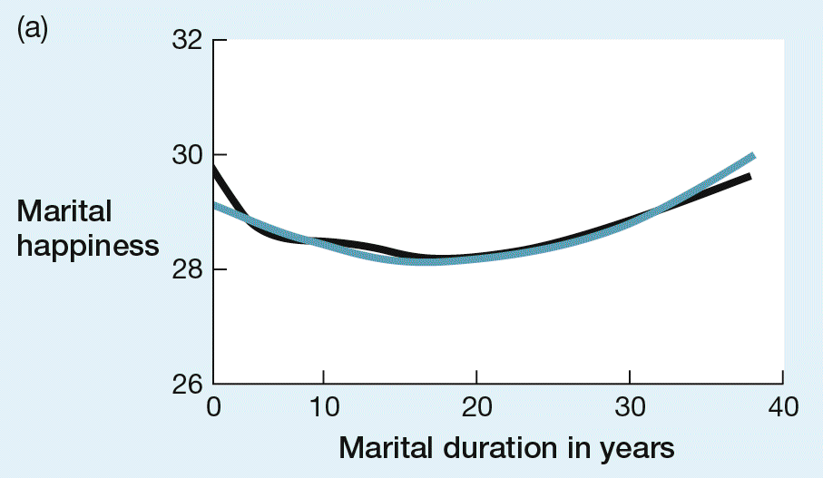
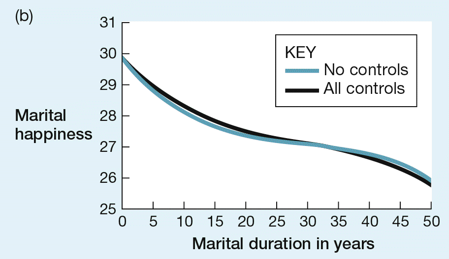
FIGURE 3.5 How marital satisfaction changes over time. (a) A cross-sectional analysis suggests that marital happiness is highest in early marriage, declines in the middle years, and then rises again in the later years. (b) Longitudinal data reveal the U-shaped curve to be an illusion: Marital happiness on average declines more or less evenly over time. (Source: VanLaningham, Johnson, & Amato, 2001.)

The problem with this conclusion was that none of these early studies had examined change at all. As a number of researchers were quick to observe (e.g., Spanier, Lewis, & Cole, 1975), even though couples married a long time tend to be happier than couples who have been married less time, marital satisfaction does not always increase in later marriage. These critics speculated that the results might be a consequence of attrition bias: The least happy marriages may dissolve early, leaving only happier couples in the long-married group.

To settle the issue, the next generation of marital researchers used longitudinal studies to examine how the satisfaction of particular couples develops over the course of their marriages. This kind of research took more time to conduct, of course, but when these studies were finally published, there was no evidence of the famous U-shaped curve. Vaillant and Vaillant (1993), for example, who followed a sample of 169 marriages for 40 years, found that satisfaction on average declined more or less evenly throughout the marriage (Figure 3.5b). VanLaningham, Johnson, and Amato (2001) followed couples for merely 8 years but were able to describe how marital satisfaction changed over that time in marriages of different duration. These researchers also found that, regardless of whether they looked at early marriage, middle marriage, or late marriage, satisfaction tended on average to decline over time. In study after longitudinal study, the results have been consistent: No U-shaped curve, no increases in later marriage, just a more-or-less steady decline.

The difference between the U-shaped curve, which was conventional wisdom in the field for many years, and the actual pattern of change in marital satisfaction illustrates the importance of designing studies that are appropriate to the questions being asked.

Another disadvantage of longitudinal research is that, as with all correlational research, the conclusions that can be drawn are limited. Compared to cross-sectional studies, longitudinal studies do get somewhat closer to supporting causal statements, because a cause has to precede its effect. For example, if a longitudinal study shows that difficulty resolving problems predicts whether a couple will break up within 2 years, the conclusion that problem-solving skills lead to relationship stability is more plausible than the conclusion that relationship stability leads to problem-solving skills. But even when a variable precedes a result in time, that variable does not necessarily cause the result. In trying to understand the effects of problem-solving skills over time, longitudinal research alone cannot determine whether such skills themselves create more stable relationships, or whether some third variable associated with problem-solving skills (such as relationship satisfaction) is the real culprit. Although longitudinal research is well suited for describing how relationships change and for predicting relationship outcomes, explaining them—and in particular, drawing strong conclusions about what causes them—requires a different kind of research design.

Experimental Research

To understand not only what happens and when it happens, but also why things happen in relationships, researchers must go beyond passively observing how different variables correlate. In experimental research, they take a more active role by manipulating one element of a phenomenon or situation to determine its effects on the rest. If changing one part while holding the rest constant consistently leads to a particular result, researchers are justified in concluding that the part that was manipulated causes the result.

Conducting an experiment requires four elements: a dependent variable, an independent variable, control, and random assignment. To illustrate the importance of each of these, let’s consider a classic experiment by social psychologists Karen Dion, Ellen Berscheid, and Elaine Hatfield (1972). During the late 1960s and early 1970s, a wave of research revealed the powerful role physical appearance plays in romantic attraction. In this study, the researchers explored why we tend to like people who are physically attractive. They wondered whether the mere fact that someone is visually appealing leads to other positive judgments about that person, even those that are logically unrelated to appearance (Figure 3.6). Because their question focused on cause (physical appearance) and effect (positive judgments), they chose to explore it by conducting an experiment.

FIGURE 3.6 Does beautiful mean good? In animated cartoons, heroes and villains are often distinguished by their appearance. Can you separate the good guys from the bad guys in animated movies just by looking at them? What lessons does this convey to an audience?

The starting point in every experiment is the dependent variable—the effect or outcome the researchers want to understand. In the attraction study, participants viewed three photographs of people and rated their impressions of each one (Dion et al., 1972). For example, they had to guess each person’s personality, predict which one was most likely to be happily married, and indicate what kind of job each person might have. These ratings were the dependent variables. They are called “dependent” because their value may depend on other aspects of the experimental situation—in this case, the physical appearance of the people in the photos.

That which is striking and beautiful is not always good, but that which is good is always beautiful.”

—Ninon de L’Enclos, French author and courtesan (1620–1705)

If the dependent variable is the possible effect, the independent variable is the possible cause—the aspect of the experimental situation the researcher manipulates, changing it “independently” of any other aspect to see if changes in the independent variable are associated with changes in the dependent variable. In the Dion et al. study (1972), the independent variable was the physical attractiveness of the people in the three photos.

How can a researcher manipulate something like physical attractiveness? Before the study began, the researchers had asked 100 college students to rate the visual appeal of 50 yearbook photos. Once they found three images of people consistently rated as highly attractive, moderately attractive, and unattractive, they presented participants with one of the photos, thereby manipulating the attractiveness of the individuals the participants would view (the independent variable). The researchers observed that when the person in the photograph was more attractive, participants’ judgments of that person were significantly more positive; compared to the less attractive people, participants rated the more attractive people as more well adjusted, more likely to have a satisfying marriage, and more likely to have a prestigious job.

Could the research team now conclude that physical attractiveness causes positive judgments about people? Not yet. Perhaps there were other reasons for the differences they observed. What if the more attractive photos were in color and the less attractive ones were in black and white? Maybe people rate any color photograph more positively, regardless of physical appeal. What if the images in the more attractive photographs were all male, and those in the less attractive photographs were all female? Maybe people generally rate men more positively than women. To support the idea that physical attractiveness, and not any other variable, really had an effect, the researchers had to rule out any alternative explanations for their observations. Doing so requires researchers to control, or hold constant, all aspects of the experimental situation they are not manipulating.

In the Dion et al. (1972) study, the researchers were interested only in the effects of physical attractiveness, so they had to control every other way the three photos might vary. Using yearbook photos helped accomplish this control because they are all the same size, and each person’s head fills about the same amount of the frame. They also made sure the participants saw either three males or three females, thereby controlling for any differences in ratings associated with gender. Because the three pictures were alike in every way other than facial attractiveness, the researchers were more justified in concluding that differences in attractiveness caused the differences in how the photos were rated.

Even though researchers can control almost every aspect of an experimental situation, they cannot control the research participants. Every person who participates in a survey or an experiment brings a unique set of prejudices and experiences that represent a final threat to the conclusions of an experimental study. Suppose, for example, that rather than using the same three photographs, the researchers had shown different photos to different groups of people. If the group who saw the photos of the most attractive people also made the most positive judgments, would that mean attractiveness affected the ratings? Maybe, but as an alternative, perhaps the group who saw the photos of the most attractive people was somehow more generous or more optimistic than the group who saw the other photos.

How can researchers ever hope to rule out these alternatives, when they cannot control the research participants? The solution is random assignment, which guarantees that every research participant has an equal chance of being exposed to each version of the experimental manipulation (the independent variable). For example, suppose participants were randomly assigned to view images of a very attractive, a moderately attractive, or an unattractive person. There would be no reason to expect that, on average, the members of any one group are different from the other two groups. Within any group, the participants vary randomly, so all their prejudices and experiences cancel each other out. If the three groups still differed in their judgments of the photos, the researchers could be reasonably sure that variations in the images, rather than preexisting differences in the groups, accounted for the varying judgments.

Pros and Cons A well-designed experiment reveals how manipulating one variable may affect a change in another variable while controlling for other possible sources of influence. Therefore, experimental research enables investigators to move beyond description and prediction to address explanations about intimate relationships. What features make people more or less attractive to friends and romantic partners? Does a particular kind of therapy or program help relationships or harm them? To explain causes and effects, an experiment is the most appropriate research design.

The increased control required in experimental research does have its costs. Isolating the effects of specific variables risks distorting how those variables behave in the world outside the experiment. In the Dion et al. (1972) study, participants were asked to make sweeping judgments about the people they saw only in photographs. Do the effects of visual appeal in this situation mirror the way physical attractiveness works in the real world? Maybe not. When we meet people in real life, we can withhold our impressions until we’ve interacted with them, or change our evaluation based on our experiences with them. By itself, the fact that physical appearance affected judgments in this experiment doesn’t mean attractiveness has the same effect when we actually meet someone versus seeing a photo.

In other words, what’s demonstrated in an experimental setting doesn’t necessarily work the same way in the real world. Experimental researchers often argue about the issue of external validity—whether the results of an experiment apply in other situations, or generalize to different contexts. Naturally, researchers hope their experiments will have high external validity and that the effects they observe will apply to a wide range of people in a wide range of situations. The more factors a researcher controls and manipulates, however, the less the experimental situation resembles other situations and the more external validity is threatened.

A broader limitation arises when what researchers want to study is difficult or impossible to control, and conducting an experiment is not an option. This is especially true for intimate relationships, in which subjects of great interest—such as relationship history, abuse, and sexual orientation—simply cannot be manipulated. Researchers would like to make causal statements about how each of these variables affects intimate relationships, but because they can’t manipulate or control them, they can’t conduct experiments that would support such statements scientifically. Perhaps due to this problem, experiments make up a relatively small part of research on intimate relationships.

Archival Research

It is possible to address interesting and important questions about relationships without gathering a speck of new data. In archival research, the researcher examines existing data that have already been gathered, usually for an unrelated purpose, by someone else. Psychologist Avshalom Caspi and his colleagues, for example, have taken advantage of archival data to study how personality—something usually described as pretty stable across the lifespan—may change over time in married couples. One set of studies addressed whether spouses become more similar to each other over time, and if so, why this might occur (Caspi & Herbener, 1990; Caspi, Herbener, & Ozer, 1992). To explore these questions, the researchers might have conducted a longitudinal study, gathering a sample of married couples and following them for several years to see if their personalities grew more similar or less similar to each other. This study design would have been appropriate, but expensive and time-consuming.

Instead, these researchers drew upon three studies that had mostly been conducted before any of them were born. Two of these were the Berkeley Guidance Study and the Oakland Growth Study, both longitudinal projects that contacted children in the late 1920s and early 1930s and then followed them periodically for their entire lives. The third was the Kelly Longitudinal Study, a project that contacted couples who were engaged in the late 1930s and followed them for 40 years. None of these projects was designed with the goal of studying how personality changes or remains stable in marriages. Still, the data from these studies were rich enough that they could be used to address a variety of questions that had never occurred to the original researchers. Caspi et al. (1992), for example, were able to draw upon these studies to show that married people’s personalities tend to remain relatively constant across their lives, in part because they tend to marry spouses who are similar to themselves. Due to the great expense of contacting families, researchers who collect data on families often ask more questions than needed for exploring the specific issues under study. By doing this, they’re establishing the potential for later archival research.

Besides revisiting existing data, archival researchers generate new data from archival sources that may never have been intended for use in research. For example, college yearbooks contain pages and pages of valuable data on people’s physical appearance, at least from the shoulders up. Social psychologists LeeAnne Harker and Dacher Keltner (2001) took advantage of these data to examine how women’s facial expressions in their yearbook photos predicted their marital status 30 years later (Figure 3.7). They found that the more positive the facial expressions in the yearbook photos, the more likely the women were to be married at age 27; and for those who remained married, the more satisfied they were with the marriage at age 52. These findings are powerful evidence for the role that a positive outlook can have across the lifespan.

FIGURE 3.7 Reading the future in a face. College yearbooks are treasured mementos, and for psychologists they can also be a source of archival data. In this study, women who had a positive expression in their yearbook photo were more likely to be happily married 30 years later. (Source: Harker & Keltner, 2001).

Personal advertisements are another potential goldmine for archival researchers. To examine differences in the qualities that straight or gay people look for in a mate, psychologist Doug Kenrick and his colleagues analyzed the features mentioned in personal ads seeking same-sex and different-sex partners (Kenrick, Keefe, Bryan, Barr, & Brown, 1995). In this study, as in most archival research that draws from public documents, the features the researchers wanted to examine were not initially presented in a form they could analyze. As a result, archival researchers often need to conduct a content analysis, by coding the materials in such a way that they can quantify and compare their differences. Harker and Keltner (2001), for example, rated the degree of positivity of the expressions in their yearbook photos on a scale of 1 to 10. Kenrick et al. (1995) calculated, for each of their personal ads, the difference between the stated age of the person placing the ad and the age of that person’s desired partner. In this way they revealed that, regardless of their sexual orientation, men tend to seek out partners younger than themselves; but women, regardless of their sexual orientation, are more accepting of partners their own age or older. Content analysis of archival materials is similar to coding observational data because it raises similar challenges of deciding what dimensions to code and establishing reliability among coders.

Pros and Cons Archival researchers are the recyclers of science. They wring new information from old data sets and find new truths, sometimes literally in other people’s trash. When questions can be explored using archival data, this approach is economical and effective. It is often more efficient than, and just as accurate as, conducting an entirely new study. To study historical trends, or to examine how variables were associated in the past, researchers often have no alternative but to conduct archival studies. As new analytical strategies and theoretical approaches are developed, the possibility of doing archival research means that any data ever collected may still contain new insights—if not today, then in the future.

Limitations to archival research reside less in the study design than in the data themselves. Because archival researchers don’t gather the data to be analyzed, they can’t control the quality of the information. If the original study was of poor quality, the archival research will be of poor quality as well. Similarly, the design of an archival study depends on the design of the original data. If the original data are cross-sectional, a reanalysis years later will still be cross-sectional and will be limited to addressing the questions that cross-sectional data can answer.

A final limitation of archival research, and an especially frustrating one in terms of intimate relationships, is that the researcher can examine only the questions asked in the original study. Caspi and his colleagues wanted to understand how personality changes or remains stable across the lives of married couples (Caspi & Herbener, 1990; Caspi et al., 1992), and they could do so only because the designers of the studies they drew from had thought to include personality measures. If new theories and concerns suggest new questions that have not yet been asked in existing studies, then archival research—as economic and efficient as it may be—is nevertheless ruled out.

Which Research Design Is Best?

Table 3.4 compares the features of correlational, longitudinal, experimental, and archival research. We can now look at which research design is the best. As the table makes clear, the most appropriate design for any study depends on the questions being asked. If you want to know what relationships are like, correlational research is perfectly suited to describing different aspects of intimate relationships and how they are associated. Describing how relationships change, or predicting whether and when they will end, calls for longitudinal research. Understanding why relationships change and determining cause and effect require an experiment. Archival research, although rarely used for experiments, is an option for either cross-sectional or longitudinal research, depending on how the original data were collected. In every case, when the study design is tailored to the questions being explored, then the strengths of the design bolster confidence in the study conclusions.

Table 3.4 Comparing Research Study Designs

	General Approach	Advantages	Disadvantages
Correlational (cross-sectional) research	Assesses several variables on a single occasion	Can describe naturally occurring associations among variables	Cannot support causal statements
Longitudinal research	Assesses variables on more than one occasion	Can describe change over time and predict outcomes	Cannot support causal statements; attrition bias
Experimental research	Evaluates the effects of an independent variable on a dependent variable in a controlled setting	Can support causal statements	Results may not generalize outside the experimental situation
Archival research	Reanalyzes existing data originally gathered for another purpose	Cost-effective and can provide historical perspective	Conclusions are limited by the quality of the original data

Table alternative text: A matrix comparing research study designs by their approach, advantages, and disadvantages.

MAIN POINTS

• Correlational research examines the naturally occurring associations among variables; it can be either cross-sectional, measuring all variables at a single occasion, or longitudinal, collecting data from the same individuals several times.
• Examining causal effects requires experimental research, in which participants are randomly exposed to different manipulations of an independent variable and all other variables are controlled.
• Archival research involves reexamining existing data that may have been collected for another purpose; it can be used to explore descriptive or predictive questions.

Glossary

• correlational research
  A research design that examines the naturally occurring associations among variables; used for answering descriptive questions.
• causation
  The capacity of one event or circumstance to directly produce a change in another.
• cross-sectional data
  In correlational research, data that have been collected at one time; they describe a cross-section, or a snapshot, of a single moment.
• longitudinal research
  A research design that collects measurements from the same participants on two or more occasions; used for answering descriptive and predictive questions.
• daily diary approach
  A longitudinal research design in which participants provide data every day at about the same time.
• experience sampling
  A longitudinal research design in which data from participants are collected throughout the day, thereby capturing thoughts, feelings, and behaviors close to when they occur.
• attrition bias
  In longitudinal research, a bias caused by participants dropping out, leading to a final sample that differs from the initial sample in important ways.
• experimental research
  A research design in which researchers manipulate one element of a phenomenon or situation to determine its effects on some outcome or predicted consequence; used for examining questions of explanation and causation. See also dependent variable; independent variable.
• dependent variable
  In experimental research, the effect or outcome the researchers want to understand. See also independent variable.
• independent variable
  The element of an experiment the researcher manipulates, changing it “independently” of any other aspect of the situation to determine whether changes in this variable are associated with changes in the dependent variable.
• control
  In an experiment, the holding constant of all aspects of the experimental situation that are not being manipulated.
• random assignment
  A way of guaranteeing that every research participant has an equal chance of being exposed to each version of the experimental manipulation.
• external validity
  The extent to which results obtained in an experimental setting generalize to different contexts.
• archival research
  A research design in which the researcher examines data that have already been gathered by someone else, often for an unrelated purpose.
• content analysis
  The process of coding open-ended materials in order to identify and quantify important phenomena.