Chapter 5
Fixed-Income Return Analysis
Price is what you pay. Value is what you get.
Warren Buffet
Chapter 5 extends the valuation framework presented in Chapter 4 to return analysis. The metrics presented in Chapter 3 are often referred to as parametric because they represent a set of measurable factors that define a fixed-income security and may be classified as either valuation measures related to the price or risk of a fixed-income security.
- The valuation measures that define the price of a bond are:
- The yield to maturity
- Nominal spread to the coupon curve
- Spread to the spot rate curve (zero volatility OAS)
- Option-adjusted spread (OAS)1
- The risk measures that define the price risk of a bond are:
- Effective duration and effective convexity
- Key rate duration and key rate convexity
5.1 Return Strategies
Individually, neither the valuation measures nor the risk measures provide a sense of the expected return of a fixed-income security. Return analysis combines both the valuation and risk measures to inform the investor of a fixed-income investment's potential return profile given her expectation of the future evolution of interest rates.
At first blush, one may argue that return analysis is not pertinent to the buy-and-hold investor since the investment horizon is equal to the maturity of the bond, which is not the case for the following reasons:
- First, for a buy-and-hold investor, the holding period return or terminal value is dependent on the future path of interest rates because the investor must reinvest coupon income at the prevailing market rate—which more likely than not will be different from the yield to maturity assumption used to price the bond, subjecting the buy-and-hold investor to reinvestment rate risk. Generally speaking, the longer the holding period, the greater role of the reinvestment rate in determining the investor's horizon return.
- Second, the investor for any number of reasons may be “forced” to sell prior to maturity under an adverse interest rate environment resulting in a principal loss. Alternatively, the investor may be “forced” to sell under a favorable interest rate environment resulting in principal gain.
- Finally, asset allocation strategies often look to the relative return of one asset class versus another to determine the proper allocation between any number of potential investments. Return analysis is a critical input to the asset allocation decision.
Aside from the buy-and-hold strategy discussed above, return strategies may be classified in one of two ways [Waring and Siegel 2006]:
- 1. Total rate of return strategies are relative strategies in the sense that the return of the asset under consideration is measured relative to the return of others. For example, the return of bond A may be measured against that of bond B, or a prescribed performance benchmark index, or liability stream as in the case of portfolio immunization strategies. The goal of a total return strategy is to “beat the benchmark,” thus generating excess return, or alpha. In the total return case, negative returns are acceptable so long as they are less than that of the relative benchmark.
- 2. Absolute return strategies shun the concept of a performance benchmark to measure alpha. The absolute return investor's strategies are designed to seek a positive return under any market condition. The goal is to produce a consistent return that is above that of the market return—alpha. For example, a stated return of 1-month LIBOR plus 250 bps would represent the goal of an absolute return investor. The absolute return investor, unlike the total return investor, may take a short position against a comparable long position to capture alpha.
The above descriptions illustrate that the differences between a buy and hold, total return, and absolute return investor are those of the investment time horizon and/or the direction of the position taken by the investor (i.e., long or short). Both the buy-and-hold and total-return investors are by definition long only investors. The difference between these two investors is their investment time horizons. Specifically, a total return investor typically has a shorter horizon than that of the buy-and-hold investor. The absolute return investor differs from the total investor only in the sense that she may take a short position against a long position in an attempt to capture alpha. Conversely, the total return investor is long only, seeking to create alpha against a specific performance benchmark.
5.2 The Components of Return
There are three components to the return realized by the fixed-income investor:
- 1. Coupon income—the interest rate that is paid to the investor for lending the money to the borrower.
- 2. Reinvestment income—the income earned through the investment of the coupon income.
- 3. Price change—the appreciation or decline (principal gain or loss) of the fixed-income security relative to its purchase price.
5.3 The Buy-and-Hold Strategy
The following example illustrates the buy-and-hold return analysis, the simplest of the three return strategies discussed above. Consider a 3.0% five-year bond priced at par to yield 3.0% to maturity. To understand how the coupon and reinvestment income components contribute to the investor's total return, Table 5.2 presents a return matrix. The return matrix allows for the systematic calculation of the investor's horizon total return. The assumptions used in the return analysis matrix are:
- The investor reinvests her cash flow receipts to match the time to the next coupon payment. In this case, six-month intervals.
- The reinvestment rate is assumed to be constant at 0.25% (25 basis points).
- The investor's holding period is to maturity (implicit in the buy-and-hold strategy).
5.3.1 Coupon Income
The investor receives coupon income, which is calculated by multiplying the bond's coupon by the principal balance outstanding at the time of the last payment date. The coupon accrues according to the bond basis that is one of the following:
- Actual days/Actual days
- 30 days/360 days
- Actual days/360 days
Table 5.1 shows the timing of the investor's expected coupon income. In this case, she expects to earn $150 of coupon income over her anticipated holding period.
Table 5.1 Return Matrix Input—Coupon Income
| 1 | 2 | 3 | 4 | 5 | 6 | 7 | 8 | 9 | 10 | Total |
| $15 | $15 | $15 | $15 | $15 | $15 | $15 | $15 | $15 | $15 | |
| Coupon Income | $150 | |||||||||
Table 5.2 Return Matrix: Coupon Income plus Reinvestment
| 1 | 2 | 3 | 4 | 5 | 6 | 7 | 8 | 9 | 10 |
| $15 | $15.04 | $15.08 | $15.11 | $15.15 | $15.19 | $15.22 | $15.26 | $15.30 | $15.34 |
| $15 | $15.04 | $15.08 | $15.11 | $15.15 | $15.19 | $15.22 | $15.26 | $15.30 | |
| $15 | $15.04 | $15.08 | $15.11 | $15.15 | $15.19 | $15.22 | $15.26 | ||
| $15 | $15.04 | $15.08 | $15.11 | $15.15 | $15.19 | $15.22 | |||
| $15 | $15.04 | $15.08 | $15.11 | $15.15 | $15.19 | ||||
| $15 | $15.04 | $15.08 | $15.11 | $15.15 | |||||
| $15 | $15.04 | $15.08 | $15.11 | ||||||
| $15 | $15.04 | $15.08 | |||||||
| $15 | $15.04 | ||||||||
| $1,015.00 | |||||||||
Total Coupon  Reinvestment Reinvestment |
$151.70 | ||||||||
| Coupon Income | $150.00 | ||||||||
| Reinvestment Income | $1.70 | ||||||||
| Return of Principal | $1,000.00 | ||||||||
| Total Return | $1,151.70 | ||||||||
5.3.2 Reinvestment Income
- In the first period, the investor receives her scheduled coupon payment of $15 and reinvests it at the six-month rate of 25 basis point annually.
- In the second period, she receives her next coupon payment of $15 and the maturation of her reinvestment of the previous coupon payment of $30.01875.
- In the third period, she again receives her next scheduled coupon payment of $15 as well as the return of her reinvestments, a total of $45.06.
The investor's annualized return is given by the following:
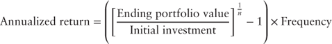
where:  |
= | Number of periods |
| Frequency | = | Payment frequency of the bond |
The investor's annualized return in this example above is:
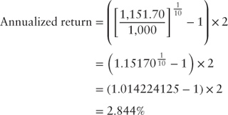
- Initially, one may notice that the annualized holding period return to maturity (2.844%) is not equal to the bond's yield to maturity (3.0%). The difference is because the short-term reinvestment rate of 0.25% is considerably less than the yield to maturity. Yield to maturity is an internal rate of return calculation and as such assumes the cash flows are reinvested at the internal rate of return (section 3.2). More often than not, this assumption is violated. Cash flows may be reinvested at a higher or lower rate, depending on the path of future interest rates.
- Furthermore, in this example the reinvestment income contributes very little to the investor's overall return, which is typically the case, particularly when interest rates are low or the horizon period is short.
5.4 Total and Absolute Returns
Unlike the case of the buy-and-hold investor, the total or absolute return investor may sell her bond investment prior to maturity. In the case of either the total or absolute return investor, the holding period is generally shorter than the maturity of the bond. Indeed, even a buy-and-hold investor may be required to sell her investment in order to raise cash to meet an unexpected out flow from the portfolio. As a result, a price change that is due to a change in the yield maturity as well as a shorter time maturity, due to the passage of time, affects her realized holding period return.
5.4.1 Price Change
The price change is given by the following:
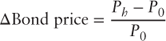
where:  |
= | Horizon price |
 |
= | Initial investment price |
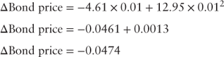
Revisting equation (3.11):

the modified duration of a five-year, 3.0% bond is 4.61 and its convexity is 12.95. Thus, given an instantaneous (+/−) 100 bps change in the term structure the expected price change of a 3.0% five-year bond priced at $100 is 4.74%.
The duration and convexity profile of a bond indicate the bond's price risk given a change in the term structure. However, that profile does not indicate the return an investor may expect to realize, given a holding period that is shorter than the bond's maturity date.
5.5 Deconstructing the Fixed-Income Return Profile
The return analysis presented in this section continues with the hypothetical yield curve used in Chapter 3 and is presented again in Table 5.3. Given an investment horizon that is less than the time to maturity of the bond, the expected return is calculated using equation 5.1.
Table 5.3 Hypothetical Swap Rate Curve
| Tenor | 1-yr. | 2-yr. | 3-yr. | 5-yr. | 10-yr. | 20-yr. | 30-yr. |
| 1.00% | 1.50% | 1.75% | 2.15% | 3.00% | 3.60% | 3.75% |
The assumptions used are:
- A 3.0% five-year bond priced at par.
- Yield to maturity is 3.0%.
- The nominal spread over the five-year benchmark is 85 basis points.
- A holding period (investment horizon) is two years.
- The nominal spread on a comparable three-year bond is 65 bps.
Two years forward, assuming both the swap curve and nominal spreads are unchanged the price of the bond is $101.72875. The pricing inputs are:
- A three-year maturity bond with a 3.0% coupon.
- The yield to maturity is 2.40% (1.75% + 0.65%).
- The price of a three-year, 3% coupon bond two years forward yielding 2.40% is $101.72875.
What is the investor's realized return? From Table 5.2, the coupon income plus reinvestment (two years) is equal to $60.23. The price of the bond increased $101.72875. The investor's proceeds from the sale of the bond after two years is equal to $1,017.2875 plus the coupon and reinvestment income, totaling $1,077.517.
From equation 5.1 the investor's annualized return given a two-year holding period assuming that the swap curve remains unchanged is:
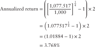
Given a two-year horizon, the investor's realized annual return is more than that which would have been achieved under the buy-and-hold strategy due to the following:
- In all, the yield to maturity declined 60 basis points from the time of the initial investment, raising the price of the bond:
- First, the bond price went up because it is priced relative to the three-swap rate, a lower yielding benchmark than the five-year swap rate that was used at the point of the initial investment.
- Second, the nominal spread also fell from 85 bps to 65 bps, a decline of 20 bps.
- However, the reinvestment rate, 25 bps, is lower than that assumed by the yield to maturity calculation (3.0%), which reduces realized income.
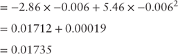
The metrics used to describe the risk of the bond also changed at the two-year horizon. The duration and convexity of the bond at the end of the two-year horizon are 2.86 and 5.46, respectively. Substituting the change in the yield to maturity, the horizon duration, and the horizon convexity into equation 3.11 yields a predicted price change:
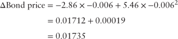
Using the risk measures of duration and convexity observed at the end of the two-year investment horizon and given the swap curve presented in Table 5.3 the estimated change price is 1.735%, close to the observed price change of the bond at the end of the two-year horizon.
Together, the measures that define the price of a bond and those that define the risk of a bond can be used to estimate the return of a bond given an investment horizon, a horizon yield to maturity, and the horizon duration and convexity.
5.6 Estimating Bond Returns with Price and Risk Measures
The estimated return is calculated by using equation 1.5 and assuming a annual reinvestment rate of 25 basis points as illustrated in Table 5.2. The return attributable to both coupon and reinvestment income is:

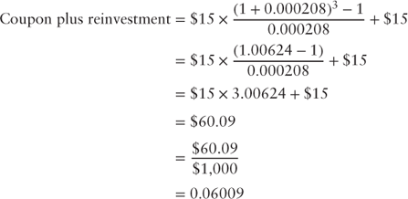
In the above example, the investor received a three-payment annuity of $15 and a final payment at the horizon date of $15. The total coupon income plus reinvestment income received by the investor at the end of the two year horizon is $60.09. The estimated price change at the end of the two-year horizon assuming the swap curve presented in Table 5.1 is given by the following:

The investor's holding period return is 7.74%. The investor's estimated annualized return is 3.76%. The example above illustrates an important point; individually the measures that define price or risk tell the investor little about the expected return of a fixed-income security. However, together they provide the investor with some insight regarding the expected return over a given investment horizon. Return analysis examines each of the three components of total return presented in section 5.2.
- Coupon income: In the simplest sense the investor may consider the coupon income as an annuity.
- Reinvestment income: The income generated by reinvesting the coupon income. To estimate the reinvestment income the investor may assume a constant reinvestment rate—a flat term structure assumption. Alternatively, the investor may assume a reinvest rate that follows the forward rate curve—a non-linear term structure assumption.
- Price change: The gain or loss realized by the investor due to a change in the price of the bond over the investment horizon. It is determined by the principal balance outstanding at the end of the investment horizon and pricing the security based on the simulated changes the level, steepness, and curvature of the term structure as described in section 4.3 and illustrated throughout the previous chapter. Both sections 5.2.3 and 5.2.4 show that the price change based on the given scenario is determined by rolling the security forward.
Return analysis blends the measures that define both the price and risk of a bond to provide the investor with an understanding of its expected return given the following inputs:
- The investor's holding period.
- A term structure assumption at the end of the holding period.
- A reinvestment assumption over the holding period.
- In the case of an MBS or ABS security, a prepayment assumption.
Return analysis allows the investor irrespective of her strategy (buy and hold, total return, or absolute return) to assess the return potential of a fixed-income security. Indeed, using this analysis she is able to select a portfolio that meets her unique risk/reward profile regardless of the strategy that she chooses.