Chapter 9
The Predictive Prepayment Model
Those who have knowledge, don't predict. Those who predict, don't have knowledge.
Lao Tzu, 6th Century Chinese Poet
Chapter 9 extends the concepts presented in Chapter 8 and presents a framework for the implementation of a predictive residential mortgage voluntary prepayment model. Unlike the semi-parametric model outlined in Chapter 8 the predictive model presented in this chapter is parametric. It assumes a structural functional form of  and an underlying error structure. The nature of a parametric model allows it to reliably predict outcomes beyond those presented within training data space used to tune “fit” the model.
One may ask, why a parametric model? Indeed, regression splines or piece-wise polynomials may fit the data much better. However, there are two drawbacks to these techniques:
- There is a risk of “overfitting” the model to the data.
- Predictions outside the training data space may not be reliable.
On the other hand, a parametric model may not perform as well as a semi-parametric model within the training space. However, this drawback is mitigated by the following qualities:
- A parametric model greatly reduces the risk of overfitting the data.
- The model will perform reliably (extrapolate) outside the training data used to fit its parameters.
From statistical standpoint, a prepayment model, or any predictive model, must be “parsimonious and robust,” meaning that the model should use the fewest predictor variables (parsimonious) to explain as much of the variation in the data as possible (robust).
The base Bond Lab® prepayment model is a parametric model. Mortgage prepayment modeling is a time to failure problem that naturally leads to the application survivorship modeling. The base line hazard is:

The influence of borrower incentive is included into the model as an multiplicative term:

Functionally, the model is:
9.1 Turnover
The investor may choose to model turnover either as a function of predictor variables or simply assume a long-term average turnover rate as presented in section 8.6.2.1. In both cases, it is apparent that the prepayment model takes the form of an exponential survivorship model in that  , the baseline survival function is housing turnover. For the sake of simplicity, the Bond Lab® prepayment model assumes an average turnover rate of 6%, which translates to an SMM of 0.5143%.
9.2 Loan Seasoning
The Bond Lab® prepayment model incorporates a three parameter asymptotic function [Crawley 2013]. The function is a multiplier on the estimated turnover rate and given by:

where:  |
= | The function's asymptote |
 |
= | The intercept |
 |
= | The point of maximum curvature |
9.2.1 Tuning Loan Seasoning Parameters
Given that the seasoning function is multiplicative on the housing turnover rate  (the asymptote) is by definition 1.0. Figure 8.9 suggested the first month prepayment rate begins around 1.0 CPR. Thus,
  is calculated as follows:

Estimating the parameter for  is more complex. The point at which the seasoning ramp is rising most steeply (
 ) is around 3.6% CPR at month 6. Rearranging terms,
  is given by:

The tuning parameters  = 1.0,
  = 0.879, and
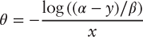
  = 0.192 result in the seasoning ramp presented in Figure 9.1.
- The seasoning ramp begins at 1.0% CPR in the first month.
- Prepayments increase over the next 29 months and reach a maximum of 6.0% CPR in month 30.
Figure 9.1 Loan Seasoning
9.3 Seasonality
Mortgage prepayments follow the home selling season in that they increase in the spring and summer months then decline in the fall and winter months. The seasonality function is given by the following equation [Spahr and Sunderman 1992] and shown in Table 9.1.
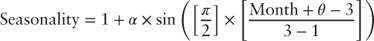
where:  |
= | tuning parameter setting the function's maximum value |
 |
= | tuning parameter setting the point at which the function reaches its maximum value |
Table 9.1  Model Parameter
 |
1 | 2 | 3 | 4 | 5 | 6 | 7 | 8 | 9 | 10 | 11 | 12 |
| Mo. | July | June | May | Apr | Mar | Feb | Jan | Dec | Nov | Oct | Sep | Aug |
9.3.1 Tuning the Seasonality Parameters
The seasonal factors presented in Table 9.2 are calculated using the National Association of Realtors existing home sales data. The data were obtained from the Federal Reserve of Saint Louis's FRED database and covers the period between January 1999 and April 2014. The seasonal factors are calculated using the R package decompose.
- The one-month CPR values presented in Table 9.2 are those of “at-the-money” loans. For this analysis, an at-the-money loan is defined as a loan whose note rate is within 20 bps of the prevailing mortgage rate lagged by two months. Constraining the analysis to the “at-the-money” borrower removes the refinancing component and the remaining quantity is housing turnover (
 ).
). - Observations are grouped by calendar month. The reported prepayment rate is the average rate realized in each calendar month across the data set. Simple division of each month's CPR by the average yields a crude estimate of the mortgage prepayment seasonal component.
- Notice, the average “at-the-money” prepayment rate is 8.2 CPR, which is consistent with the housing turnover analysis presented in Figure 8.7. The pattern of the seasonal factors, although somewhat different, is consistent with the seasonal pattern presented in Figure 8.10.
Table 9.2 Seasonals
| Month | CPR | Seasonal |
| Jan | 9.8 | 0.87 |
| Feb | 8.5 | 0.86 |
| Mar | 8.0 | 0.87 |
| Apr | 7.4 | 0.93 |
| May | 6.5 | 1.00 |
| June | 8.3 | 1.08 |
| July | 8.6 | 1.13 |
| Aug | 8.4 | 1.15 |
| Sep | 8.9 | 1.12 |
| Oct | 9.6 | 1.07 |
| Nov | 6.9 | 0.99 |
| Dec | 8.0 | 0.91 |
| Average | 8.2 |
Based on the analysis presented in Table 9.2, the initial values chosen for the parameters  and
and  are 0.15 and 12, respectively. Figure 9.2 compares the function estimate to the seasonal factors calculated using the R package decompose. The seasonality model follows the expected seasonal pattern. The model's forecasted prepayment rate increases in the spring and summer months and declines in the fall and winter months.
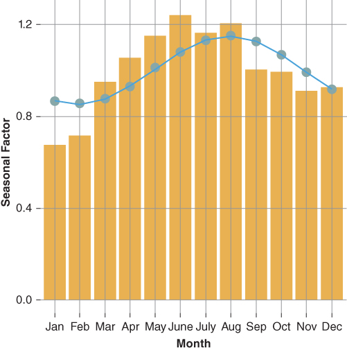
Figure 9.2 Model vs. Actual Seasonals
9.4 Borrower Incentive to Refinance
Chapter 8 illustrated that the homeowner's response to a refinancing incentive is a sigmoid or S-shaped function. Any number of parametric functions representing an S-curve to model the borrower's incentive to refinance may be used. The Bond Lab prepayment model implements an arc tangent function with both a slope and location parameter. Incorporating these two parameters provides a more flexible borrower response function than the basic arc tangent function. The Bond Lab borrower incentive function is given below:
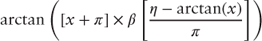
where:  |
= | borrower incentive |
 |
= | an integer that defines the slope of the response function |
 |
= | a numeric parameter that defines the location of the response function |
- Figure 9.3 shows that decreasing the value of
 (i) increases the slope of the function as well as increasing (decreasing) the maximum (minimum) values of the arc tangent response.
 - Figure 9.4 shows that negative values of
 (n) shift the arc tangent response to the left while positive values shift the arc tangent response to the right.
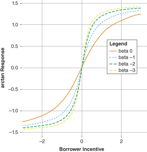
Figure 9.3 Slope
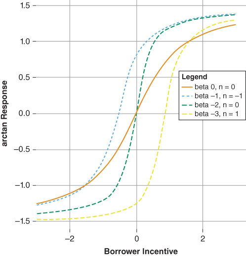
Figure 9.4 Inflection
Together, Figures 9.3 and 9.4 illustrate that equation 9.8 provides sufficient flexibility to model a borrower's response to a given refinance incentive. The complete borrower incentive function is given by equation 9.9:

The arc tangent function approaches  as
as  and
and  as
as  . Thus:
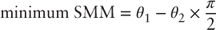
and,
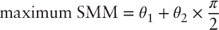
Solving for  and
and  yields the following:
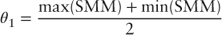
and
Tuning the model to the data presented in Figure 8.5 yields the following initial estimates of  and
and  .
.
 ,
, 
Next, provide an estimate for  as follows:

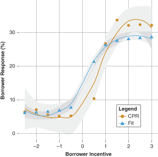
The estimated slope coefficient is −2.67. Finally, provide a location estimate. Generally, a good starting point is somewhere between 0 and 1.0. To begin,  . The borrower's incentive response model shown in Figure 9.5 fits the “shape” of the data well. However, the model tends to overestimate the “out of the money” prepayment rate while underestimating that of the “in the money” prepayment rate. The results of the initial parameters suggest shifting the incentive curve to the right (increasing
  as well as increasing the slope
  ). Furthermore, increasing both
  and
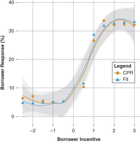
and  should increase the overall predicted borrower response to changes in the prevailing mortgage rate. Figure 9.4 illustrates how changes to
  (−6),
(−6),  (0.75) as well as adjustments to both
  (0.019) and
  (0.01) improved the overall fit of the borrower response function.
 ,
, 
9.5 Borrower Burnout
The term burnout refers to the evolution of the composition of borrowers within a pool of securitized mortgage loans. Burnout is the attempt to capture the diversity of these borrowers (i.e., the heterogeneity of the pool) and how the pool's borrower diversity influences the investor's realized prepayment rate. In order to capture the diversity of the borrowers within a pool of mortgage loans, the analyst must make assumptions about the characteristics of those borrowers [Stanton 1995] [Hayre 2006]. The two most important and commonly used modeling assumptions center around the following concepts:
- Refinance velocity, which is related to a borrower's response to a given refinancing incentive as described in section 9.4. A borrower may be classified as either a fast payer or a slow payer. A fast payer is a borrower that exercises his option to refinance efficiently while a slow payer is one that does not [Hayre 2006].
- Adverse selection, which refers to a borrower's refinancing cost. Typically, those borrowers with a stronger credit profile and consequently a lower cost to refinance exit the mortgage pool sooner, leaving behind those borrowers with a weaker credit profile [Stanton 1995].
It is important to note that the burnout variable does not specify the transition of borrowers from fast payer to slow payer or vice versa, but rather, the change in the composition of the borrowers within the pool as time passes. That is, burnout refers to the migration of borrowers out of the MBS pool rather than the migration of borrowers within the MBS pool. Some have argued that using loan level data to predict prepayment rates eliminates the need to incorporate a burnout variable. This argument is untenable because the analyst does not possess a priori knowledge of borrowers' propensity to prepay; hence, a burnout variable is required. The presence of a burnout variable in the model allows the analyst to observe borrower behavior over time and adjust the composition of the pool or loan level borrower profile with respect to exhibiting either fast or slow payer behavior given the borrowers' response to recurring refinancing incentives. In the case of loan level data, a burnout variable serves to assign a probability to a borrower's tendency to exhibit either fast payer or slow payer behavior for a given economic incentive to refinance.
Figure 9.7 illustrates how borrower response to a given refinancing incentive changes over time. Using FHLMC's loan level data, a loan is classified based on time from origination (loan age) as follows:
- New: The loan's age is less than or equal to 36 months. A new borrower exhibits a stronger propensity to refinance given that he has recently closed a loan and may require little preparation in terms of documentation. In addition, he is likely aware of prevailing mortgage rates and as a result more likely to refinance. Furthermore, there is little chance of a negative credit migration due to a life event such as a job loss, divorce, of business failure.
- Moderate: The loan's age is between 37 and 60 months. The moderately seasoned borrower exhibits a weaker propensity to refinance. The borrower may simply be unaware of refinancing opportunities or reluctant to assemble the required paperwork need to document the loan throughout the underwriting process. Given the passage of time, the borrower may have experienced a life event that may have resulted in a negative credit migration, which may increase the cost associated with refinancing.
- Seasoned: The loan's age is greater than 60 months. The seasoned borrower exhibits the weakest propensity to refinance. The longer the borrower maintains his loan, the greater his reluctance to refinance. This is due to potential extension of the term of loan, as well as the cost associated with the refinance relative to the loan's current balance.
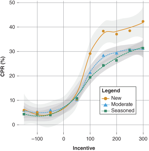
Figure 9.7 S-curve by Loan Seasoning
In addition to the above:
- Figure 9.7 suggests that the pool's maximum refinancing response rate declines over time as the loan age increases (seasons) as fast payers exit the pool leaving behind the slow payers.
- Finally, Figure 9.7 illustrates that the “refinancing elbow” or the inflection point of the S-curve shifts to the right, an indication that a greater percentage of slow payers are represented in the MBS pool relative to the fast payers. This is classic definition of MBS pool burnout.
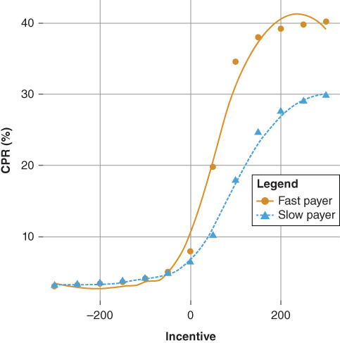
Figure 9.8 S-curve Fast and Slow Payer
Together, the above suggests that over time the composition of the cohort has shifted as the fast payers exit the pool leaving behind the slow payers. Burnout is also path dependent [Hayre 2006]. The complete path of rates may also be incorporated into the burnout equation. Typically, the rate path component of the burnout variable measures the maximum incentive forgone by the borrower. Decreasing  increases the baseline rate of burnout while increasing
  slows the burnout.

| where: Incentive | = |  |
The burnout function used by Bond Lab recognizes the influence of both the passage of time as well the path of mortgage rates. Figure 9.9 illustrates the behavior of the burnout variable given  tuning coefficients between −0.01 and −0.05 and holding
  at 0. The baseline burnout implies that the pool begins with a composition that is 100% fast payers. Higher values of
  implies a slower rate of burnout.
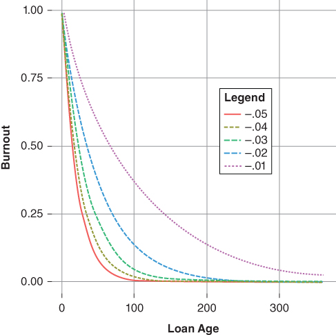
Figure 9.9  Burnout
Figure 9.10 holds  constant (−0.01) and increases
  from −0.05 to −0.01. As the borrowers in the pool forgo successively greater refinancing opportunities, the probability that these borrower's are fast payers declines and the expected borrower response rate converges to that of the slow payer. Thus, the burnout variable defines the composition of pool of MBS with respect to the relative percentage of fast versus slow payers.
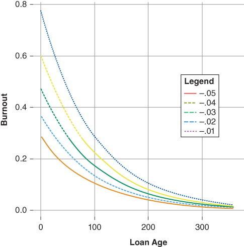
Figure 9.10  Burnout
In the case of a loan level prepayment model, the burnout variable does not measure the transition of a borrower from that of a fast payer to a slow payer but, rather, revises the posterior probability that the borrower is a fast payer. The burnout variable incorporated into the Bond Lab prepayment model interpolates the composition of pool of mortgages or a borrower's propensity to exhibit either fast or slower payer behavior. The burnout equation extends the borrower incentive equation 9.9 as follows:

where:  |
= | Fast payer S-curve |
 |
= | Slow payer S-curve |
| Burnout | = | Burnout variable |
The modeling challenge is to find the initial tuning parameters such that given a zero incentive the borrower incentive function presented in 9.14 does not add to the baseline turnover assumption. The following steps tune the initial parameter estimates of the Bond Lab model to a 8% CPR turnover assumption, a 0.0069 SMM.
- First, tune the model's baseline seasoning ramp (equation 9.4) such that the seasoning ramp reaches its peak in 30 months. The loan seasoning parameters are
 = 0.879 and
  = 0.192 (section 9.2).
 - Second, establish the model's minimum fast and slow payer SMM. The Bond Lab prepayment model is additive on the baseline SMM.
- Given the data presented in Figure 9.7 the “out of the money” (minimum) CPR is 3%, 0.00254 SMM, subtracting the baseline assumption yields an initial minimum of incentive of −.0043
- Third, tune the model's fast and slow payer “in the money” maximum SMM.
- The model assumes a fast pay maximum rate of 60% CPR. Deducting the base case turnover rate of 8% CPR yields a maximum fast payer SMM of 0.067%. The astute reader may recall from Figures 9.6 and 9.7 the actual maximum refinance CPR was around 40%. If this is the case, why choose 60% CPR? Recall, we are tuning a fast payer refinance response and the data represent the average refinance response across all payers—that is, burnout is embedded in the data.
- The model assumes a slow pay maximum rate of 25% CPR. Deducting the base case turnover rate of 8% CPR yields a maximum slow payer SMM of 0.017%.
- Using equations 9.9 through 9.11, determine the initial tuning parameters for the fast and slow payer S-curves.
- Table 9.3 summarizes the final tuning parameters for both the fast payer and slow payer S-curves. The tuning parameters set the minimum and maximum incentive SMM of the S-curve net of the model's assumed baseline turnover rate. Additionally, the initial tuning parameters are set such that given a 0-basis-point incentive, the S-curve is neutral on the turnover rate. The fast and slow payer tuning parameters are given in Table 9.3.
- Finally, tune the burnout parameters. The burnout parameters are set initially such that the composition of fast and slow payers are estimated at pool issuance and revised based on the pool's observed prepayment behavior. In the case of a loan, the parameters are set to reflect the investor's belief that the borrower is either a fast or slow payer at loan origination. To begin, the incentive parameter is set at 25 basis points, reflecting the investor's view of the fast payers' refinance threshold, which is the minimum incentive needed to motivate a fast payer to refinance. The initial burnout tuning parameters are given in Table 9.4.
Table 9.3 Fast, Slow Payer Tuning Parameters
| Min SMM | Max SMM |  |
 |
 |
 |
Location | |
| Fast Payer | −0.0043 | 0.067 | 0 | 0.031 | 0.023 | −4.41 | 1.0 |
| Slow Payer | −0.0043 | 0.017 | 0 | 0.064 | 0.002 | −0.66 | 0.5 |
Table 9.4 Burnout Tuning Parameters
 |
 |
Incentive |
| −0.01 | −0.01 | 25 |
Figures 9.11 through 9.14 illustrate each element of the Bond Lab prepayment model given the initial tuning parameters.
- The loan seasoning multiplier increases over 30 months to its asymptote (1.0).
- The seasonality multiplier is representative of the home selling season, reaching a crest of 1.15 in August and its through 0.85 in February.
- The borrower incentive function (equation 9.14) reflects the expectations of fast and slow payer behaviors. Both the fast and slow payer functions are tuned such that they are neutral, a 0% SMM, on the turnover component of the model when the borrower's note rate is equal to the prevailing mortgage rate—no incentive to refinance.
- The burnout variable is tuned to reflect the investor's view of the pool'scomposition of fast and slow payers. In the case of a loan level model, burnout is the probability that the borrower is a fast payer.
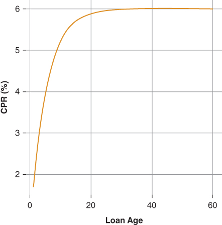
Figure 9.11 Loan Seasoning Multiplier
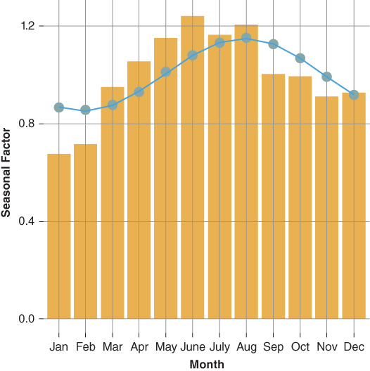
Figure 9.12 Seasonality Multiplier
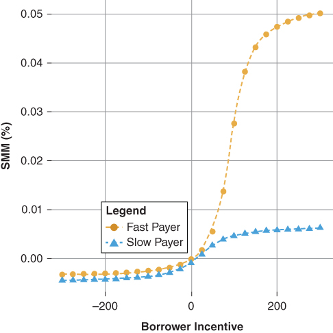
Figure 9.13 S-curve Fast/Slow Payer
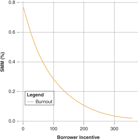
Figure 9.14 Burnout
The Bond Lab® mortgage prepayment model represents the basic infrastructure used in prepayment modeling and easily extends to include additional variables. The initial tuning parameters result in a model that assumes the percentage of fast-payer borrowers in a pool is around 78%, the model's maximum refinance CPR is 60% and the minimum “out-of-the-money” CPR is 3%.
Figure 9.15 presents the results of the final model assuming the mortgage rate is unchanged (the borrower's incentive is 0). The model seasons over 30 months and the expected prepayment range is between 8% and 6% CPR depending on the application of the seasonal factor. The burnout variable controls both the rate, through the age variable, and the extent to which the mortgage pool's composition changes from fast to slow payers via the burnout variable—note in the example burnout is held constant and as a result expected prepayments are a function of loan seasoning and seasonality. Alternatively, in the case of a loan level model, the burnout variable estimates the probability that the borrower is a fast or slow payer.
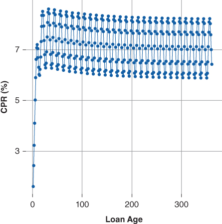
Figure 9.15 Bond Lab® Mortgage Prepayment Model
9.6 Application of the Prepayment Model
Recall the following from Chapter 8:
- Stratification of the Cox model on loan purpose suggested that the survivor function of loans originated for purchase, refinance, or cash-out were significantly different from one another.
- Stratification of the Cox model on loan age yielded a significant improvement of the model's fit.
The first suggests the investor may tune the Bond Lab prepayment model to each loan purpose, implying three different models each predicting prepayment rates based on loan purpose. The burnout variable includes a time element, which reduces the need to stratify the model over loan age. By tuning three models to loan purpose, the overall predictive ability of the combined models improves by as much as 0.8% CPR.
9.6.1 Additional Variables Influencing Mortgage Prepayment Rates
Adding additional variables that may explain borrower behavior will likely improve the model. For example, some borrower characteristics that may increase the cost (friction) to refinance include:
- Home price inflation/deflation
- Credit score
- Debt-to-income ratio
- Loan-to-value ratio
- Origination channel
- Loan size
- Loan term
- Note rate type—fixed, adjustable, hybrid
Each of these variables can cause greater or less refinancing friction for the borrower. For example, a borrower with a lower credit score, all else equal, will experience a higher refinancing cost in terms of rate, documentation, and mortgage insurance than a borrower with a higher credit score. In addition, the combination of variables may also alter a borrower's propensity to prepay his mortgage. Consider a borrower with a high credit score, low debt-to-income ratio, and high loan-to-value ratio. How would each of these borrower characteristics come together to influence the borrower's expected prepayment rate?
The origination channel (retail, correspondent, or broker) may influence prepayment rates.
- A retail origination is performed directly by the lender. The retail channel is often referred to as a bricks-and-mortar because the loan is originated in one of the lender's branch offices. Lenders are often reluctant to solicit retail borrowers to refinance due to the potential impact of higher observed prepayment speeds on their servicing portfolio valuation or, in the case of a lender that relies on securitization for term funding, a higher cost of funds charged by the investor.
- A correspondent is a loan broker with an exclusive arrangement with a lender. The correspondent originates a loan in accordance with the lender's underwriting guidelines. The correspondent's relationship with the lender generally deters the correspondent from soliciting the borrower for a subsequent refinance.
- A broker is independent of an exclusive origination agreement and “sells” closed and funded loans to any number of lenders. As a result, the broker is likely to solicit borrowers to refinance when the borrower is “in-the-money.” Consequently, broker-originated loans tend to exhibit slightly faster prepayment rates than those originated through either the retail or the correspondent channel.
The loan size, or original balance, also influences prepayment rates. The costs associated with refinancing a loan are both fixed and variable. Examples of fixed costs are [Governors of the Federal Reserve System no date]:
- Attorney and legal fees ($500–$1,000).
- Title search and insurance fees ($700–$900).
- Property Inspection fee ($175–$350).
- Survey fee ($150–$400).
Relative to the original balance of the loan, the fixed fees represent a greater percentage of the cost to refinance increasing the borrower's friction. As a result, a borrower with a lower balance requires a much lower mortgage rate to refinance than does a borrower with a higher mortgage balance.
Table 9.5 illustrates the influence of loan balance on the refinancing decision. A borrower with an original balance of $100,000 refinancing from a 5% mortgage rate to a 4.5% mortgage rate would recover the fixed costs in 66 months. Conversely, a borrower with an original balance of $400,000 refinancing from a 5% mortgage rate to a 4.5% mortgage rate would recover the fixed costs in 16 months.
Table 9.5 Refinance Analysis by Original Balance
| Orig. Bal. | Mtg. Pmt. 5.0% | Mtg. Pmt. 4.5% | Saving | Fixed Cst. | Mos. to Recover |
| 100,000 | 536.82 | 506.69 | 30.14 | 2,000 | 66 |
| 150,000 | 805.23 | 760.03 | 45.20 | 2,000 | 44 |
| 200,000 | 1073.64 | 1,013.37 | 60.27 | 2,000 | 33 |
| 250,000 | 1342.05 | 1,266.71 | 75.34 | 2,000 | 26 |
| 300,000 | 1610.46 | 1,520.06 | 90.41 | 2,000 | 22 |
| 350,000 | 1878.88 | 1,773.40 | 105.48 | 2,000 | 18 |
| 400,000 | 2147.29 | 2,026.74 | 120.55 | 2,000 | 16 |
The loan term and note rate type also influence borrower prepayment rates. Typically, a borrower with stronger credit and greater financial flexibility will choose a 15- over a 30-year amortization term, implying the 15-year borrower may demonstrate a greater propensity to refinance than his 30-year counterpart.
The type of note rate chosen also indicates the borrower's propensity to refinance. A borrower may choose an adjustable rate or hybrid (a mortgage with an initial fixed rate followed by an adjustable rate) mortgage for its lower relative starting payment versus a standard fixed-rate mortgage. In turn, the borrower might be motivated to refinance when the loan's rate resets depending on the general level of interest rates and the slope of the yield curve.
Together, Chapters 8 and 9 outlines Bond Lab's analysis and predictive model of mortgage prepayment rates. Chapter 9 provides the basic framework for any prepayment model as wells as Bond Lab's base case model tuning parameters for a FHLMC 30-year “generic” loan or pool. The investor's prepayment model plays an important role in the valuation of mortgage-backed securities. There is not a single Bond Lab “prepayment model” but, rather, a library of prepayment models each of which is tuned to reflect the investor's expectation of future borrower behavior. In order to model residential mortgage prepayment rates, the investor employs both semi-parametric and parametric modeling techniques. Based on the insights gleaned from the semi-parametric analysis, the investor must then decide which, if any, borrower and/or loan characteristics upon which to stratify her library of prepayment models.