1
A Primer to Flooding, Razing and Watersheds

It may seem strange to devote an entire book about image processing to flooding and watershed basins. Does this rather limited and anecdotal subject deserve such an extensive mathematical treatment? This introductory chapter will convince readers of the merits of reading and studying this book.

Lakes and catchment basins are familiar concepts, as we may observe them in any mountainous relief. Floods, especially cataclysmic ones make the headlines of the television.

In fact, a grey tone image corresponds to each topographic relief, if we assign to each spatial position a gray tone proportional to the altitude of the relief. Inversely, considering the gray tones of a gray tone image as altitudes turns the image into a topographic relief. The concepts developed for topographic reliefs are thus easily transposed to images and vice versa.

In this chapter, we affine our perception of these topographic structures and show in how many different ways they intervene in the field of image processing, for filtering or segmenting images.

1.1. Topographic reliefs and topographic features

1.1.1. Images seen as topographic reliefs and inversely

A topographic relief is fully defined if an altitude corresponds to each location of a domain. If we represent this altitude as a gray tone between 0 and a maximal value Max, we get an image called the digital elevation model. Such digital elevation models may be derived from satellite images observing the Earth. Figure 1.1(a) shows on the left-hand side a three-dimensional (3D) representation of a topographic relief, in which several rivers dug deep gorges in the surrounding mountains. The gray tone image on the right-hand side is a digital elevation model (DEM) representing the same topographic relief. The highest points in the relief correspond to the brightest points in the image. The rivers appear as dark lines crossing the image.

Inversely, each gray tone image may be considered as the digital elevation model of a virtual topographic surface. For instance, if we negate the DEM of Figure 1.1(a), replacing each gray tone λ with the gray tone (Max – λ) (where Max represents the maximal gray tone, i.e. to the white color), we obtain a new DEM and a new topographic relief shown in Figure 1.1(b). This topographic relief does not exist in nature, but conveys a better understanding of the structure of the rivers than the initial topographic surface of Figure 1.1(a).

Figure 1.1(c) has no relation at all with a topographic surface as it shows an angiography of the human retina, with the vessels of the retina appearing white. This image is very similar to Figure 1.1(b). Again, the 3D representation on the left-hand side of Figure 1.1(c) presents the vessels of the retina as a topographic surface.

As we have extensive experience in interpreting landscapes, it is worthwhile developing our ability to consider images as landscapes.

A landscape may be submitted to all sorts of transformations: a new volcano may appear, large areas are flooded, the level of the sea increases and submerges some atolls, etc. We will also transform the images using particular operators. An operator defines how to compute the new gray tone value at each location of an image or altitude in a landscape as a function of the values taken by nearby values. For instance, we will define an operator called erosion, which assigns to each location the darkest gray tone met in the vicinity. The negation of a gray tone image is an example of an operator that only considers the gray tone λ at a given location and replaces it with the gray tone (Max – λ).

If the domain is one dimensional, we have a signal. The spatial domain may be the time, and the gray tone represents any measurement.

The domain of definition of the images may take any number of dimensions. A 3D solid object may be represented as a 3D binary function, taking the value 1 inside the solid matter and 0 outside. Figures 1.24(a) and (c) show a foam and a 3D object, respectively. It appears here as a binary image in a 3D domain. Figure 1.24(b) shows the gray tone distance of each voxel to the boundary of the object, and Figure 1.24(d) shows the labels of the various cells of the foam which have been reconstructed; both these images are gray tone images.

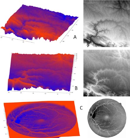
Figure 1.1. a) A real topographic surface, represented as a relief on the left and as a digital elevation model on the right-hand side. b) A topographic surface which does not exist in reality. The preceding relief has been turned upside down; the digital elevation model being the negative of the preceding one. c) Angiography of a human eye on the right-hand side and its representation as a topographic surface on the left-hand side. For a color version of the figures in this chapter, see www.iste.co.uk/meyer/topographical1.zip

1.1.2. Topographic features

1.1.2.1. Catchment zones, regional minima and flowing paths

In this primer on morphology, we focus on catchment zones and lakes of a topographic relief. We define these entities in an intuitive way, without any mathematical developments. These will appear later, in the technical part of the book.

The catchment zones are related to the trajectories of a drop of water falling on a topographic relief. Such a drop of water follows a line of swiftest descent and ends in a zone from where it cannot escape, as there is no way for it to go further downwards. This ultimate destination is a flat zone of the topographic surface or a lake. A drop of water falling on a flat zone or plateau spreads out on the plateau until it reaches a lower border of the plateau from where it may resume its gliding down. Figure 1.2(a) shows a topographic surface and a drop of water falling on the surface. The arrow shows the trajectory of this drop downwards, towards a regional minimum. The lines of the steepest descent followed by a drop of water are called flowing paths. A point may be the origin of several flowing paths, leading to only one or several distinct regional minima.

The catchment zone of a regional minimum is the set of points from where a flowing path starts and leads to this minimum. Catchment zones overlap if they contain points linked with distinct regional minima by distinct flowing paths. Later in this book, we present methods for reducing or suppressing the overlapping of catchment zones, producing the so-called watershed partitions.

Figure 1.2(a) shows a topographic relief with 10 regional minima. A catchment zone is associated with each of these minima. In this particular example, the catchment zones do not overlap and form a partition. Each region is highlighted by a different color below Figure 1.2(a).

1.1.2.2. Lakes

Lakes are simply connected zones covered by water. The surface of the lakes is of course flat. The topographic surface covered by a lake vanishes completely, replaced by a flat area. For this reason, a flooded topographic surface is more regular than the same, unflooded surface.

A lake that is impossible to quit without climbing is surrounded on all its boundaries by points with a higher altitude. Such a lake is a regional minimum lake. Adding a drop of water inside slightly increases its level, without provoking an overflow.

On the contrary, adding a drop of water to a full lake provokes an overflow, as a flowing path exists that is able to quit the lake towards points with a lower altitude.

1.1.2.3. Catchment zones of flooded reliefs

The presence of lakes on a topographic relief deviates flowing paths. The regional minima of a flooded topographic surface are dry or are lakes. In both cases, a drop of water falling on such a regional minimum is trapped in this minimum. If it falls elsewhere, it will follow a flowing path until reaching a regional minimum. This flowing line may follow a line of swiftest descent when it falls on dry ground. If it falls on a full lake, it will quit the lake by one of its exhaust points, creating an overflow, which continues its way downwards. It may cross several full lakes, always escaping by an exhaust point before reaching lower ground.

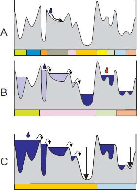
Figure 1.2. The catchment zones associated with the various ways of flooding a topographic surface. The watershed partition is situated below each topographic surface, with different colors assigned to each tile. a) An unflooded topographic surface, in which all regional minima generate a catchment zone. The trajectory of a drop of water is highlighted. b) On this flooded topographic surface, there remain four regional minimum lakes. All others are full lakes and belong to the catchment zone of a regional minimum lake. Adding a drop of water to a full lake provokes a cascade of overflows, until reaching a regional minimum lake. c) A similar situation to that in B. This particular flooding is the highest flooding for which the regional minima marked by a vertical arrow remain dry. It contains two regional minima

Figure 1.2(b) shows what happens when a drop of water falls on a flooded relief. The red drop falls inside a regional minimum lake, slightly increasing the level of the lake. The blue drop of water falls inside a full lake, provoking an overflow of a drop of water. This drop of water follows a flowing path, reaches another full lake, provokes another overflow, etc. After the final overflow from a full lake, the drop of water follows a final flowing path and reaches a regional minimum lake.

In Figure 1.2(b), only four regional minima remain. The first one, starting from the left, does not contain a lake. The three others, in dark blue, contain regional minimum lakes. The associated watershed partition now also contains four regions, for each regional minimum. The new basins result from the merging of basins of the unflooded relief in Figure 1.2(a).

After filling a number of catchment zones with full lakes, only a restricted number of regional minima remain. Their catchment zones are unions of catchment zones of the initial relief. Flooding a topographic relief has thus a powerful regularization effect.

1.1.3. Modeling a topographic relief as a weighted graph

1.1.3.1. Node weighted graphs

A topographic surface is defined on a continuous domain. In order to represent its DEM in a computer, we have to define it on a regular grid. Each picture element (or pixel) of the grid is assigned a numerical value representing a gray tone value. Such an image may be modeled as a node-weighted graph. The pixels of the grid are the nodes of the graph. Neighboring pixels of the grid are linked by an edge of the graph. The gray tone attributed to a pixel in the image is attributed to the node of the graph. Thus, we are able to represent each gray tone image, in any dimension, defined on any grid as a node-weighted graph. This model correctly represents a gray tone image in any dimension, but is much more general. A family of objects on which a binary relation, taking the values true or false, is defined may be represented by a graph. The nodes of the graph represent the objects; two nodes of the graph are linked if the binary relation between the corresponding objects is true. If we furthermore assign a weight to each node, we obtain a gray weighted graph.

1.1.3.2. Edge-weighted graphs

Alternatively, the nodes may be unweighted, but the relations between the nodes may be more or less intense. If two nodes have no relation at all, then they are not linked by an edge. If a relationship exists between them, then they are linked by an edge with a weight expressing the intensity of this relation. Consider, for instance, a geographic map, in which each country is modeled by a node. Two neighboring countries are linked by an edge. The weight of the edge may be any measurement, for instance, the volume of economic exchange between the two countries. As another example, the nodes of the graph may represent chemicals, the edges expressing the intensity of the reaction between chemicals if such a reaction takes place.

1.1.3.3. The topography of a weighted graph

Graphs are abstract structures. We will characterize the topography of graphs as we would characterize the topography of a relief, by observing the trajectory of a drop of water deposited on the relief. Such a drop of water follows a line of swiftest descent before reaching a regional minimum, i.e. a flat zone from without lower neighbors in which the drop of water remains trapped. All nodes linked by such a line of swiftest descent with a particular regional minimum (RM) form the catchment zone of this RM.

We will characterize the topography of a weighted graph in an analogous way. We consider, likewise, the fate of a drop of water deposited on a node on the graph. We define for each type of graph, be it node-weighted or edge-weighted, the trajectories a drop of water is able to follow. The final destinations are regional minima, and a catchment zone is assigned to each regional minimum.

This topic is addressed in the first part of this book.

1.1.3.4. Flooding a weighted graph

A topographic surface may be flooded. With the formation of lakes, the topographic surface becomes simpler. We will also define flooding for weighted graphs. We assign to each node a flooding level and characterize the hydrostatic equilibrium of flooding on a graph.

Edge-weighted graphs may be used for representing the relations between the regional minima of a topographic surface. Each RM is represented by a node. Neighboring nodes are linked by an edge weighted by the altitude of the pass point that is able to pass from one minimum to the next. The level of a lake covering a regional minimum depends on the levels of the pass points leading to neighboring minima. Overflow from one lake to another takes place through these pass points. The equilibrium state of all lakes with respect to the others will also be modeled.

This topic is addressed in the second part of this book.

1.1.3.5. Assessing the validity of our models

We represent real topographic surfaces as DEM, i.e. gray tone images. We then model these gray tone images as node-weighted graphs. Our modeling will be satisfactory if the regional minima, catchment zones, types and extension of lakes during flooding match those observed on the topographic surface, which has been modeled.

Similarly, the models developed for edge-weighted graphs should match the observations on real topographic surfaces represented by these models.

However, graphs have a much larger degree of generality than simply representing topographic surfaces. The concepts and tools inspired by the topography of a relief have for this reason far greater reach and applicability, thanks to rigorous mathematical treatment.

1.2. Flooding, razing and morphological filters

1.2.1. The principle of duality

The negation of a gray tone image or the inversion of the corresponding topographic relief produces a new image and a new topographic surface. Negating the negative image and inverting the inverted relief restore the initial state.

The principle of duality is based on this negation. If ψ is an operator applied to a relief f, it is possible to associate with ψ its dual operator . If C represents the negation, then = CψC. The first negation is applied to f, producing Cf. This negated relief is transformed by ψ, producing ψCf. This final result is transformed a second time, producing .

Suppose that the operator ψ fills a number of lakes of a topographic relief, following some arbitrary rule. Let us see what its dual counterpart does. Figure 1.3(a) shows a topographic surface f. It is inverted in Figure 1.3(b). The negated relief is flooded, creating a number of lakes in Figure 1.3(c). The lakes are incorporated in the relief itself, as shown in Figure 1.3(d). This last relief is inverted again, producing Figure 1.3(e). Comparison of the initial relief in Figure 1.3(a) and the final relief in Figure 1.3(e) shows that the peaks of the initial relief have been clipped and razed. If we call flooding the operator which produces lakes, then its dual counterpart is called razing.

1.2.2. Dominated flooding and razing

1.2.2.1. The highest flooding under a ceiling function

There are many different ways of flooding a topographic relief. Lakes may be present or absent at any location, and their levels may be diverse. We now present a method for specifying a particular flooding of a topographic relief. Figure 1.4(a) shows a function f representing a topographic relief in yellow. In Figure 1.4(b), a second function g ≥ f is indicated in green above the function f in yellow. In Figure 1.4(c), a number of lakes have been created, appearing in blue. This flood distribution of the function f is the highest one below the function g; g is called ceiling function for this particular flooding. Some of these lakes are full lakes (they are identified by <norm>, standing for “non-regional minimum”), and the others are regional minimum lakes (identified by <rm> standing for “regional minimum”). The regional minimum lakes are characterized by the fact that their level is blocked by the green ceiling function g. They touch the ceiling function at some locations. The full lakes, on the contrary, do not touch the ceiling function, and their level is only constrained by the level of their exhaust point. They cannot be higher: adding a drop of water produces an overflow.

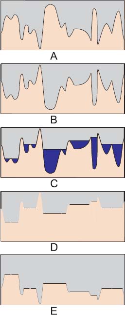
Figure 1.3. a) Initial topographic surface f. b) Mirror function O – f. c) A particular flooding Fl (O – f) of the mirror function where the lakes are highlighted. d) The same topographic surface as in C, without highlighting the lakes. e) The mirror function of the topographic function of D: Rz (f) = O – Fl (O – f)

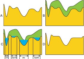
Figure 1.4. Using dominated flooding as a filtering tool: a) A topographic relief f in yellow. b) A ceiling function g ≥ f in green. c) The highest flooding of f under g creates four lakes. The lakes <mr> are regional minimum lakes, whereas the lakes <nomr> are non-regional minimum lakes. d) Filling the non-regional minimum lakes and suppressing the regional minimum lakes produce a filtered version of A, in which only the most salient wells are preserved

This method for specifying a flood distribution of f using a ceiling function g is called dominated flooding of f under g. It is extremely useful and versatile, as there are many choices for the ceiling function.

Furthermore, it helps differentiating full lakes and regional minimum lakes, which may be extracted and treated differently. In our particular example, we may chose a simplification of the topographic surface. The new surface in Figure 1.4(d) is identical to the initial surface except at the position of the full lakes, which have been filled.

By duality, we obtain the dominated razing. The dominated razing of a function f above a floor function g is the lowest razing of f above the floor level g.

More generally, most morphological operators possess a dual counterpart.

1.2.2.2. Illustration of dominated flooding and razing

Figures 1.5 and 1.6 show increasing flooding and decreasing razing of the same initial Greek mosaic. The initial image is shown on the left-hand side.

The top row of images in Figure 1.5 shows increasing dilations of the initial image (a dilation assigns to each pixel the maximal value met in a given neighborhood of this pixel; for this reason, the image becomes brighter, the bright objects expand and the dark objects shrink), serving as increasingly brighter ceiling functions for dominated flooding. The corresponding flooding is indicated below. One observes how uniform gray tone zones representing lakes become increasingly larger, covering dark details of the initial image.

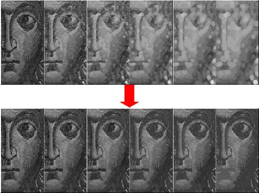
Figure 1.5. Dominated flooding associated with increasing dilations serving as ceiling images. The top row shows the ceiling functions obtained by increasing dilations. The bottom row shows the corresponding dominated flooding

Similarly, the top row of images in Figure 1.6 shows increasing erosions of the initial image (an erosion assigns to each pixel the minimal value met in a given neighborhood of this pixel; for this reason, the image becomes darker, the dark objects expand and the bright ones shrink), serving as increasingly darker floor functions-dominated razing. The corresponding razing is indicated below. We observe how uniform gray tone zones representing the top of razed peaks become increasingly larger, suppressing bright details of the initial image.

1.2.2.3. Combining flooding and razing

Flooding and razing have a very remarkable property: they create flat zones by filling valleys with lakes and by razing summits. The remaining part of the topographic surface is left untouched and remains identical. This means that the contours associated with the simplified topographic surface are unchanged compared to the contours in the initial image. More precisely, each variation in gray tones between two neighboring pixels in the simplified image corresponds to a variation in gray tones in the initial image. The reverse is not true, as the initial relief inside the flooded or razed zones has been lost and replaced by a flat zone.

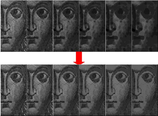
Figure 1.6. Dominated razing associated with increasing erosions serving as floor functions. The top row shows the floor functions obtained by increasing erosions. The bottom row shows the corresponding undercored razing

By concatenating razing and flooding, this property is preserved. Flooding and razing may be combined in multiple ways for simplifying images. They may be alternated, razing following flooding with increasing intensities.

Figure 1.7 shows a powerful filter obtained by alternatively razing and flooding the same image. A series of increasing functions serve as ceiling functions (High1<High2<High3…). Symmetrically, a series of decreasing functions serve as floor functions. The first razing above the floor function Low1 is followed by flooding under the ceiling function High1. The second razing above the floor function Low2 is followed by flooding under the ceiling function High2 and so on.

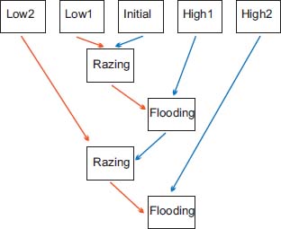
Figure 1.7. Alternate sequential razings and floodings for filtering images

Figure 1.8 shows the result of such alternate flooding and razing of the same initial image, in the leftmost position of the series. Each image is the product of flooding, followed by razing of the preceding image. From one image to the next, the intensity of flooding and razing increases. This series of images nicely illustrates how the details of the image progressively vanish, without changing the position or blurring the contours of the remaining structures.

Figure 1.8. Alternate sequential flooding and razing of increasing intensity

The levelings and flattenings are particularly interesting as they treat peaks and valleys in perfect symmetry [MEY 98b]. Levelings are obtained by the commutative product of flooding and razing.

The construction of flattenings is shown in Figure 1.9, where the function f in Figure 1.9(a) is submitted simultaneously to flooding and razing. The result is controlled by the second function g in Figure 1.9(b). Two auxiliary functions are created: the function sup(f, g) = f ∨ g in Figure 1.9(c) creates a ceiling level, whereas the function inf (f, g) = f ∧ g in Figure 1.9(d) creates a floor level. The function Fl (f, f ∨ g) in Figure 1.9(e) constitutes the highest flooding under the ceiling f ∨ g. The function Rz (f, f ∧ g) in Figure 1.9(f) is the lowest razing of f above the floor level f ∧ g. The resulting flattening of f is obtained by replacing the function f with Rz (f, f ∧ g) on the domain {f > g} and with the function Fl (f, f ∨ g) on the domain {f < g}, producing the flattened image of Figure 1.9(h).

Figure 1.9. A combination of flooding and razing in order to flatten a function f bounded by a second function _g

1.2.3. Flooding, razing and catchment zones of a topographic relief

Figure 1.10 shows the effect of flooding or razing on a real topographic surface. Figure 1.10(a) presents an initial topographic surface, submitted to an extensive flooding in Figure 1.10(b), with lakes covering large areas. Razing has clipped a number of local peaks in Figure 1.10(c). Flooding followed by razing has produced a simplified relief in Figure 1.10(d), with flattened peaks and partially filled valleys.

Finally, we have extracted the catchment zones of two minima in Figures 1.10(e) and 1.10(f). The rivers all flow out of the domain. Therefore, the lowest points of the rivers belong to the boundary of the domain. We have chosen two regional minima on the left boundary of the domain and separately extracted their catchment zones in Figures 1.10(e) and 1.10(f).

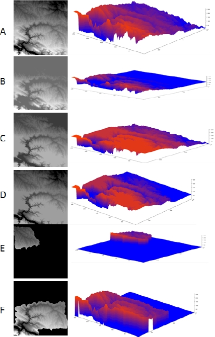
Figure 1.10. a) R = initial relief; b) flooding of R; c) razing of R; d) flooding followed by razing of R; e) catchment zone of a regional minimum; f) catchment zone of another regional minimum

1.3. Catchment zones of flooded surfaces

1.3.1. Filtering and segmenting

Flooding, razing and their combinations, leveling and flattening are powerful tools for simplifying images or their gradient before segmenting them. This preprocessing helps to obtain meaningful segmentations of images. Figure 1.11 illustrates what happens if we try to segment an image without filtering it beforehand, either the image itself or its gradient image. It represents a painting by Gauguin on which a gradient image has been computed (the modulus of the gradient at a pixel is estimated by subtracting the lowest value from the highest value of the image in a neighborhood of the pixel). As is frequently the case, this unfiltered image has many regional minima, each generating a catchment zone. The resulting watershed partition on the right has 4,888 different regions, most of them being completely insignificant.

Figure 1.11. An image (the luminance of a painting by Gauguin), its gradient image and the watershed partition associated with the gradient. This largely oversegmented partition counts 4,888 tiles

Figure 1.12 shows how this number of regions may be reduced, concentrating on the most perceptually significant regions in the image. The same initial image in Figure 1.12(a) is first filtered by alternated razing and flooding, in order to suppress noise and meaningless details as shown in Figure 1.12(b). The gradient image is then filtered by flooding it under the ceiling function of Figure 1.12(c), obtained by dilating the gradient image (in order to suppress minima with tiny catchment zones) and adding a constant value (in order to suppress minima whose catchment zone is not sufficiently contrasted). The resulting gradient image is shown in Figure 1.12(d). Its watershed partition is shown in Figure 1.12(e) in false colors. Replacing each region of the watershed partition by its mean gray tone yields Figure 1.12(f), which produces a cartoon-like representation of the initial image with only 58 regions.

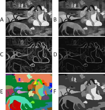
Figure 1.12. Filtering the initial image and its gradient in order to obtain sparse segmentations with a low number of significative regions: a) Initial image. b) Filtering by alternative razing and flooding. c) A ceiling function for the gradient image, obtained by dilating it and adding a constant to it. d) The flooded gradient image. e) The watershed partition of the filtered gradient image of image D. f) A mosaic image obtained by replacing each tile of the watershed partition by its mean value

1.3.2. Reducing the oversegmentation with markers

1.3.2.1. The flowing paths of a drop of water, modulated by flooding

The trajectories of a drop of water falling on a topographic relief may change dramatically when this relief is flooded. Figure 1.13 illustrates the effect of flooding on the trajectories of the flowing paths. The top row shows the real situation in which the rivers flow in the direction of the sea and quit the domain under observation at some regional minima placed on the boundary of the domain. In the next three rows, we have artificially changed these trajectories by imposing new minima after canceling the previous ones.

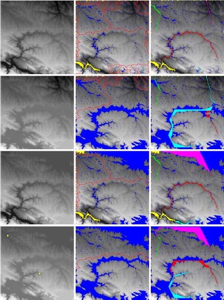
Figure 1.13. Catchment zones and flowing paths of a topographic surface if we modify the outflow points of the relief. In each row, a different outflow pattern is chosen: the complete boundary (which is the real situation) in the top row, the upper border for the second row, the left-side border for the third row and finally two yellow nodes (seen in the leftmost image) in the last row. For each row, we show the flooded topographic surface in gray on the left-hand side, in the center, the flooded zones in blue, with the limits of the catchment zones in red and the outflow points in yellow. On the right-hand side the flowing paths of marked points in the image are indicated, at identical positions in all four rows

For the second row, the minima on the upper boundary of the domain become sinks, evacuating any amount of water, all other exits being closed.

In the third row, the regional minima on the left boundary of the image are sinks, all others being closed.

In the last row, finally, we have chosen two sinks within the image as the only places through which the water may escape.

We then flood the topographic relief in such a way that the chosen sinks become active. The sinks are the only regional minima remaining in the image. A drop of water falling on the flooded topographic surface follows a flowing path, crossing lakes and dry land until it reaches an active sink. This flooding is a dominated flooding, under a ceiling function equal to 0 on the sinks and equal to the maximal altitude elsewhere. The dominated flooding has the sinks as only regional minima.

Consider now the top row, in which the sinks are all placed on the boundaries of the domain, which is the case for the real relief. However, other regional minima may exist, due either to measurement errors or they be naturally present. These minima are filled by lakes in the highest flooding, presented in blue in the second image of the row. The boundaries of the catchment zones are indicated in red. On the right-hand side, we have marked by hand several points, each with a distinct color and then followed with the same color the flowing paths starting from these points. The flowing paths nicely follow the rivers.

The situation completely changes for the next three rows. The dominated flooding is indicated on the left-hand-side image, the catchment zones of the remaining minima on the central image. The right-hand-side image shows how the flowing paths starting from the same marked points head towards the regional minima.

Flowing paths, regional minima and their catchment zones entirely depend on the position of the sinks.

Figure 1.2 shows another example of a one-dimensional topographic surface. In Figure 1.2(a), which is not flooded, there are 10 regional minima and catchment zones. In Figure 1.2(c), there remain only two regional minima, marked by an arrow. We have placed a sink at these minima, which prevents the formation of a lake at this position. We have illustrated the fate of a drop of water falling on the surface. If it falls on a lake, it provokes an overflow, such that the lake remains at a stable level. The overflowed water then reaches a new lake, provoking a new overflow and so on until it ultimately reaches a regional minimum.

This flooding may be obtained by a dominated flooding, as illustrated by Figure 1.14. The ceiling function, in orange, is equal to the maximal value, except at the position of the minima, which are to be kept, where it takes the altitude of the topographic relief. The lakes of the dominated flooding are in blue. The associated watershed partition is indicated below the figure, and it contains two regions, each around a regional minimum of the flooded surface.

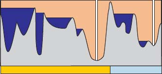
Figure 1.14. A dominated flooding of a topographic relief in which two regions are marked. The ceiling function (in orange) is equal to the relief in the marked zones, and equal to the maximal altitude elsewhere. The resulting dominated flooding has the marked regions as only regional minima, all lakes which are created are full lakes

1.3.2.2. Marker-based segmentation

In Figure 1.15, we show how to regularize the segmentation of an image by imposing markers. These markers may be hand-marked or the result of some preliminary treatment able to roughly localize the objects of interest. Figure 1.15(a) shows the initial image, and Figure 1.15(b) its filtered version. The gradient of the filtered image is shown in Figure 1.15(c). We note that this image still has many regional minima. A number of white dots are overlaid with this image, indicating the position of the markers. A dominated flooding keeps as only minima those which are marked. The contours of the resulting partition are indicated in Figure 1.15(d).

Marker-based segmentation is the process by which we flood a topographic relief in order to impose markers as the only regional minima and construct the associated watershed partition.

1.3.2.3. Segmenting cells

The next example illustrates the role of the background for segmenting fluorescent nuclei, bright on a dark background. Figure 1.16(a) shows in the initial image how the nuclei are textured with chromatin, structured in white and black dots. The gradient image appears in Figure 1.16(b). The watershed partition of the gradient image presents a severe oversegmentation in Figure 1.16(c).

For this reason, the nuclei are first submitted to alternated flooding and razing in order to suppress their texture, as shown in Figure 1.16(d). In order to obtain markers for the nuclei, we raze Figure 1.16(d), with a ceiling function obtained by eroding and subtracting a constant value from the image in Figure 1.16(d). The remaining regional maxima after the razing are then eroded and labeled, yielding the markers in Figure 1.16(e).

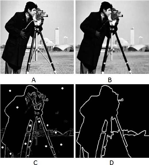
Figure 1.15. a) Initial image. b) Filtered initial image in order to smooth the textures. c) Gradient image where the white dots represent markers. d) Resulting watershed partition; each region contains one and only one marker

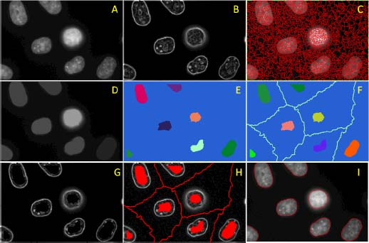
Figure 1.16. Segmentation of cell nuclei. a) Initial image. b) Gradient image. c) Contours of the watershed partition associated with the gradient image showing a severe oversegmentation, even in the background, due to the presence of low contrasted regional minima in the gradient image. d) Filtering of the chromatine structure of the nuclei using razing followed using flooding. e) inside markers of the nuclei derived from image D. f) The watershed partition of the initial image associated with the markers in image E. g) A ceiling function is constructed, equal to 0 on the markers in F and to the maximum gray tone everywhere else. The highest flooding of the gradient image is now regularized. h) The regional minima in red of the regularized gradient of G. i) The contours in red of the watershed partition of H, yielding the final segmentation

In addition, we have to produce a marker for the background. If we negate the initial image, the cells appear as dark holes. The watershed partition of this image associated with the markers of image Figure 1.16(e) is presented in Figure 1.16(f). The boundaries of the catchment basins appear in light blue, with each basin containing one marker. The image in Figure 1.16(f) now has a complete set of markers, from which we may construct a ceiling function for flooding the gradient image and obtain a new image in Figure 1.16(g), in which the only regional minima are the marked regions. The minima of this image are overlaid in red with the flooded gradient image in Figure 1.16(h). The watershed partition of this image delivers the final segmentation in Figure 1.16(i).

It is interesting to observe these images as 3D topographic surfaces. Figure 1.17(a) shows the topographic surface corresponding to the initial image in Figure 1.16(a), where the chromatin structure of the nuclei appears nicely. Figure 1.17(b) shows the gradient image of Figure 1.16(b), while Figure 1.17(c) shows the gradient image of Figure 1.16(g) after flooding.

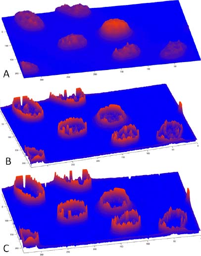
Figure 1.17. a) A 3D representation of cell nuclei. b) The gradient image of the nuclei with many minima inside and outside the cells. c) The regularized gradient image in which only one regional minimum remains in each nucleus and in the background

1.4. The waterfall hierarchy

1.4.1. Overflows between catchment basins

We again study the trajectory of a drop of water, falling on a topographic surface in order to highlight the nested structure between the catchment basins, which appears if we provoke overflows from one basin to a neighboring basin.

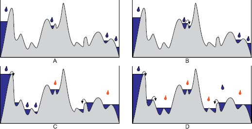
Figure 1.18. Creating critical flooding of a topographic surface: a) Creation of the four first lakes. b) The second lake is full and flows over neighboring basins, creating a new lake. c) The red drops fall into regional minimum lakes, increasing their level. The blue drops increase the level of the other lakes until they are full and flow over into a neighboring basins. d) Critical flooding: all lakes are full up to their lowest pass point. The blue drops provoke overflows of the full lakes they are falling in. The red drops fall into regional minimum lakes, whose level is increased with any additional drop of water

Figure 1.18 shows a topographic surface submitted to rain. In Figure 1.18(a), rain has started creating lakes in four basins. These basins are not full and adding a drop of water increases the level of their lakes without immediately provoking an overflow. In Figure 1.18(b), after some more rain, the level of the lakes increased. Adding an additional drop of water again increases the level of all lakes except the second lake. This lake is filled up to its lowest pass point, and a new drop of water falling into this lake provokes an overflow into a neighboring lake, which starts to be filled. In Figure 1.18(c), new lakes flow over into neighboring lakes through their lowest pass points, leading to neighboring basins. Two lakes are highlighted by the red color of the drop of water falling into them. These lakes cover two adjacent basins, filled up to the pass point separating them. The red drop of water falling in these lakes does not provoke an overflow into a neighboring lake, but rather increases their level. Both lakes constitute regional minima of the flooded surface: they are flat zones of the topographic surface entirely surrounded by points with a higher altitude.

The last image in Figure 1.18(d) shows the steady state of the flooding, where each lake is filled up to its lowest pass point. There are increases with an additional drop of water. Adding a drop of water in the others provokes an overflow into a neighboring lake with a lower altitude; this second lake may itself flow over into a third lake and so on until the final overflow occurs and ends inside a regional minimum lake.

We call critical flooding the flooding in which each lake is filled up to its lowest pass point. The serial overflows provoked by adding a drop of water to a critical flooding reveal a new structure between the catchment basins. A basin is either a regional minimum, and adding a drop of water into it slightly increases its level. Or adding this drop of water into a non-regional minimum lake provokes a series of overflows until a regional minimum lake is achieved. Thus, we define an “overflow catchment zone”, made of all basins whose cascaded overflows ultimately reach the same regional minimum lake.

This process produces a hierarchy of waterfall partitions. Level 1 of the hierarchy is the waterfall partition associated with the initial image. Level 2 contains the partition associated with the first waterfall flooding.

Level 3 is the partition associated with a new waterfall flooding from the preceding one. The process may be repeated until only one region remains, the result of merging all others.

From one level of the hierarchy to the next, new regions are merged, letting more salient regions appear.

This process is illustrated in Figure 1.19. Level 1 corresponds to the watershed partition of the unflooded topographic surface, and each regional minimum generates a watershed basin in Figure 1.19(a). The first waterfall flooding produces the lakes in blue in Figure 1.19(b). Tiny basins of level 1 enclosed in larger basins have merged in level 2. A new waterfall flooding produces new and larger lakes in Figure 1.19(c). Now, only the two most predominant basins remain, the others having been absorbed by the largest basins.

In Figure 1.20, the waterfall hierarchy has been constructed for an image of a handwritten document. The letters appear dark on a bright background. The contours between the basins appear with a shade of gray proportional to the level of the waterfall hierarchy for which they disappear. The highest levels nicely separate groups of letters and words.

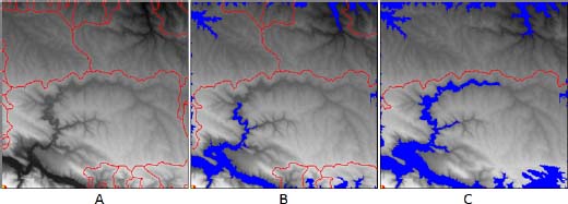
Figure 1.19. Three levels of the waterfall hierarchy: a) The initial topographic surface with the limits of its catchment basins. b) The new catchment basins after the first waterfall flooding flooded areas are in blue. c) The second waterfall flooding, the floods larger areas and the associated watershed partition now has only two regions

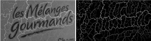
Figure 1.20. The waterfall hierarchy applied to a handwritten document. Each contour line has a gray tone proportional to the waterfall level for which it disappears. The brightest ones nicely separate letters and words

1.5. Size-driven hierarchies

The watershed partitions associated with increasing flooding form hierarchies. With higher flooding, some lakes which were previously regional minimum lakes become full lakes and their catchment zones are absorbed by the catchment zones of neighboring remaining regional minima. In the case where the flood level increases at the same rate in all of the basins, following some measurement made on the lakes (such as depth, area or volume of the lakes), the resulting hierarchies are particularly interesting.

The case when the flood progression depends on a geometrical measure of the lakes is particularly interesting. Consider, for instance, Figure 1.21 presenting four successive increasing floodings of the same topographic surface. The growth of the lakes is synchronized by their depth: at time t, all lakes have the same depth t, except the full lakes whose level cannot increase as long as the neighboring lake does not reach the same level. This is the case for the last two lakes in the second image of Figure 1.21. The last one is a regional minimum lake with a correct depth corresponding to the flooding time, whereas the neighboring lake is a full lake, with a lower depth, unable to grow as long as its neighboring lake does not reach the same level. This happens in the third figure, where both lakes have merged and have the depth equal to the flooding time. With this progression rule, the lakes remaining regional minima for the longest time are the deepest lakes. The watershed partitions are indicated by different color strokes above each flooded topographic relief in Figure 1.21.

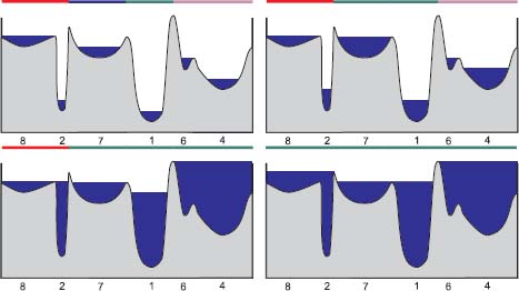
Figure 1.21. Example of a height synchronous flooding. Four levels of flooding are illustrated; each of them is topped by a figuration of the corresponding catchment basins

Other progression rules may be controlled by a different measurement on the figures. Choosing the area of the lake surface favors the lakes with the largest extensions. They will be the last ones absorbed by neighboring lakes, whereas the narrow catchment zones are quickly absorbed by neighboring regions.

Controlling the flood progression by the volume of the lakes offers an interesting compromise between the extension and the depth of the lakes.

Figure 1.22 shows an initial image and its negated gradient in the top row. Below are presented three mosaic images, with the same number of regions. Three hierarchies have been constructed, one in which the flood level is controlled by the depth of the lakes, the second by the area of the lakes and the last one by the volume of the lakes. We have chosen in each hierarchy a partition with the same number of regions. Each region is then replaced by its mean gray value measured in the initial image. The first image corresponds to the depth of the level and contains many contrasted small details. The second image, on the contrary, emphasizes the area of the regions, the small details being ignored. The last image belongs to the hierarchy controlled by the volume of the lakes and presents both types of regions, large ones and small ones if they are well contrasted.

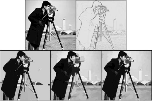
Figure 1.22. Size-oriented hierarchies. Top row: The initial image and its gradient. Bottom row: Three size-driven hierarchies have been constructed, respectively, based on the depth for the left image, the surface of the lakes for the central image and their volumes for the right image. Three particular partitions have been extracted from these hierarchies with the same number of tiles, showing that the regions that are selected largely differ according to the type of hierarchy

1.6. Separating overlapping particles in n dimensions

This overview on the usage of watersheds in image processing would not be complete without mentioning a method for separating overlapping particles in an n-dimensional domain. Figure 1.24 shows the tomography of a polyurethane foam in 3D. Such a foam is a juxtaposition of a polyhedral cell. The walls separating two cells are too thin to be visible in the tomographic view. Only the lines which are common to three adjacent polyhedral cells are visible, forming a kind of 3D skeleton of the structure. We aim to reconstruct the foils separating the cells.

The data consist of a binary image in 3D. In order to solve this problem, we construct a simpler model, made of overlapping disks in a 2D image. We try to solve this simpler problem and then extend the method to the real 3D problem to find a solution. The 2D binary model is shown in Figure 1.23(a). The key to the solution is to construct a distance function, assigning to each pixel of the binary image its distance to the lower border. Thus, as shown in Figure 1.23(b), each disk is represented by a conic gray tone shape. The summits of two overlapping disks are separated, as it also appears in Figure 1.23(c), giving a perspective view of the distance function. It then suffices to take the negative of the distance function, transforming the maxima into minima. The watershed partition of this new gray tone image nicely separates the disks, as shown in Figure 1.23(d).

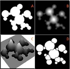
Figure 1.23. A method for separating overlapping disks in a 2D image: a) Initial binary image with overlapping spheres. b) The distance transform to the spheres. c) A 3D representation of the distance function. d) The watershed partition of the inverted distance function, separating the disks

The transposition of the solution into 3D, developed using the 2D model, is straightforward [CEN 94], [KAM 15]. Figure 1.24(b) shows the distance function to the foam skeleton shown in Figure 1.24(a). This distance function is negated, and its watershed partition constructed. The boundaries between two catchment basins form a surface spanning the foam skeleton and are shown in Figure 1.24(c). The watershed basins are assigned different gray tones and are represented as a volume in Figure 1.24(e).

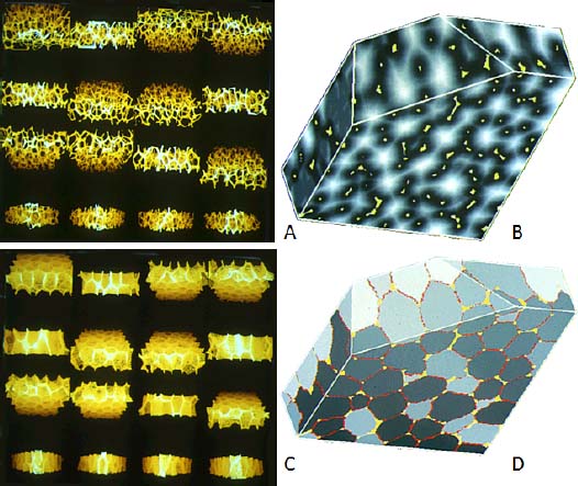
Figure 1.24. Segmentation of the 3D structure of a polyurethane foam: a) The initial binary image representing a 3D tomography of the foam. b) The distance function to the foam skeleton of A. c) The limits of the watershed partition associated with the inversed distance function. d) The resulting segmentation in which each tile of the watershed partition has been assigned a distinct gray tone, the boundaries between them being highlighted in red

1.7. Catchment zones and lakes of region neighborhood graphs

We conclude this primer on the usage of flooding and catchment zones with an introduction to graph-based morphology, which is fundamental in this book. Consider Figure 1.14(c), presenting the highest flooding of a topographic relief under a ceiling function, equal to the relief at some marked positions and equal to the maximal altitude elsewhere. It is noteworthy to remark that the level of the lakes is entirely determined by the altitude of the pass points between neighboring catchment zones of the topographic surface. In fact, only the neighborhood relations between catchment zones matter, as well as the altitude of the pass points between them. For this reason, it is more efficient to represent the topographic surface as an edge-weighted graph and to compute the dominated flooding on this graph. Figure 1.25(a) illustrates how this edge-weighted graph is created for a topographic surface. The watershed partition is placed below the topographic relief in the figure. Still below, we find the edge-weighted graph summarizing the relations between the catchment basins. Each catchment basin is represented by a node in the graph (a yellow disk in the drawing), and is identified by a letter (from a to j). The nodes are not weighted. The nodes representing two neighboring basins are linked by an edge (indicated by a red segment), weighted by the altitude of the pass point between the two basins. These weights are in red below the edges.

We denote the nodes by their letters (a, b, c, etc.). If two nodes u and v are linked by an edge, we denote the edge by (u, v) and its weight by η_uv. If a node s is flooded, we denote its flood level by τ_s.

The nodes f and j are selected as markers. They are assigned an altitude 0 (in blue inside the yellow disks). They are also assigned a label, indicated on the watershed partition, blue for the node f and orange for the node j.

The edge-weighted graph is then flooded and the progression of the flood indicated on the topographic relief itself.

The algorithm progressively expands the flooded nodes and the labeled catchment zones in parallel. We define A as the set of nodes already flooded. Initially, A = {f, j}. Each node of A obtains a different label, highlighted by a different color in the watershed partition.

The algorithm progresses as follows:

Among all edges (u, v) such that u ϵ A and , take the edge (s, t) with the lowest weight (s ϵ A and ):

label(t) = label(s)

if all nodes are labeled, stop.

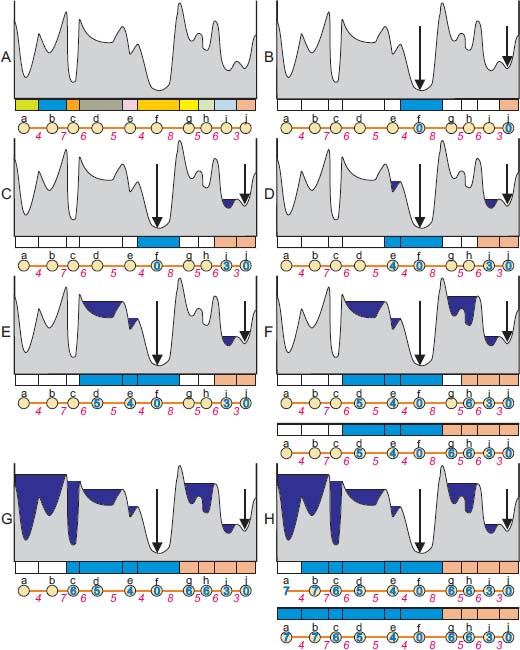
Figure 1.25. Flooding the region neighborhood graph of a one-dimensional topographic relief (see the text for the description of each step)

Let us comment the progression of the algorithm in the Figures 1.25(a): The initial topographic relief above its watershed partition, and the edge-weighted model representing the relations between its watershed basins. B: The nodes f and j are marked. They obtain distinct labels, and their watershed basins distinct color. Their flood level is set to 0: τ_f = τ_j = 0. The set A is created: A = {f, j}. C: The lowest edge crossing the boundary of A is the edge (i, j), with a weight η_ij = 3. Thus, τ_i = τ_j ∨ η_ij = 0 ∨ 3 = 3; A = A ∪ {j}; label(i) = label(j). D: The lowest edge crossing the boundary of A is the edge (e, f), with a weight η_ef = 4. Thus, τ_e = τ_f ∨ η_ef = 0 ∨ 4 = 4; A = A∪ {e}; label(e) = label(f). E: The lowest edge crossing the boundary of A is the edge (d, e), with a weight η_ef = 5. Thus, τ_d = τ_e ∨ η_de = 4 ∨ 5 = 5; A = A ∪ {d}; label(d) = label(e). F: The lowest edge crossing the boundary of A is the edge (h, i), with a weight η_hi = 6. Thus, τ_h = τ_i ∨ η_hi = 3 ∨ 6 = 6; A = A ∪ {h}; label(h) = label(i). F again: The lowest edge crossing the boundary of A is the edge (g, h), with a weight η_gh = 5. Thus, τ_g = τ_h ∨ η_gh = 6∨5 = 6; A = A ∪ {g}; label(g) = label(h).

The nodes g and h are separated by an edge with weight 5, whereas their flood level is equal to 6. Indeed, in the topographic relief, they are covered by a lake with level 6. Adding a drop of water to this lake produces an overflow into the basin i. The level of the lake is thus determined by the altitude η_hi of the pass point between the basins h and i. The flooding assigns the same altitude 6 to the nodes g and h. The node h is flooded first and τ_h = τ_i ∨ η_hi = 3 ∨ 6 = 6. The node g is flooded second τ_g = τ_h ∨ η_gh = 6 ∨ 5 = 6, the flood level of h is propagated over the pass point (g, h) with the altitude 5.

The process goes on in the next figures until all nodes have been flooded and the corresponding watershed basins are labeled. Thus, the labels of the markers have been expanded at the same time as the edge-weighted graph has been flooded, exactly corresponding to the flood propagation of the topographic relief. However, the flood propagation is much faster on the graph than on the relief, as each basin is represented by one node, whereas it occupies a large number of pixels in the corresponding topographic relief.

Figure 1.26 presents the same scenario applied to a partition in which a dissimilarity has been defined between neighboring regions. A weight is assigned to each portion of contour between two neighboring regions, expressing a kind of dissimilarity between the regions: higher weights standing for higher dissimilarities. This edge-weighted partition is represented by an edge-weighted neighborhood graph in Figure 1.26(b). Each region is represented by a node. The nodes representing neighboring regions are linked by an edge, weighted by the dissimilarity between the two regions. In Figure 1.26, two regions have been marked, highlighted by the presence of a blue pentagon. The corresponding nodes are assigned a flood level equal to 0 in Figure 1.26(c). The neighborhood graph of Figure 1.26(b) is replaced here by one of its minimum spanning trees (trees containing all nodes and of minimal total weight). This substitution will accelerate the processing as less edges are to be considered at each iteration. It is legitimate since all the edges selected at each step of the flooding algorithm above belong to the minimum spanning tree of the graph (the proof is given later in the document).

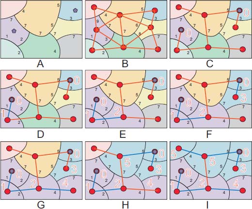
Figure 1.26. Flooding a region neighborhood graph of a two-dimensional partition (see the text for the description of each step)

In Figure 1.26(d), the first edge is considered with weight 1 and the corresponding region gets a flooding level equal to 2 and the same violet label as the marked region. The second region with a flood level of 2 is appended to the flooded domain in Figure 1.26(e). In Figure 1.26(f), the other marker expands flooding the neighboring region with yellow color, producing a lake with altitude 3. The procedure continues until all nodes have been flooded and labeled. We thus obtain a partition of the nodes, in which each region is assigned to one of the markers. If we cut the red edge in Figure 1.26(i), we obtain a forest, in which each tree spans one region of the final partition. Each tree is rooted in a marked node. The total weight of the forest is minimal. This is a well-known result: for obtaining an edge-weighted segmentation associated with a set of markers, we have to construct a minimum spanning forest in which each tree is rooted in a marker [MEY 94a].

We have presented a scenario of marker-based segmentation, which floods an edge-weighted graph and propagates the labels of the markers to all other nodes, forming a watershed partition. Thus, the circle comes back around, as the watershed partitions on images are often presented as a flooding process. Figures 1.27(a) and 1.27(b) show how an image, considered as a topographic surface, is flooded by an increasing flood starting from the regional minima of the relief [BEU 79, BEU 82, MEY 90a, BEU 90a]. The flood level in all basins is the same. In order to avoid the generation of two lakes by two distinct minima, a virtual dam (of no thickness) is erected in order to keep them separated, as shown in Figure 1.27(b). If not all regional minima serve as sources, but only a subset of them, the flood progresses differently. The flood progresses with a uniform altitude starting from the source. However, every time a lake is full, reaching a pass point leading to a basin without a source, an overflow occurs. Catchment basins without sources are thus flooded from a neighboring basin and are assigned the label of this basin. The process is identical on a topographic surface or an edge-weighted graph, as illustrated in Figure 1.26. Yet, an image or topographic surface may be considered as a node-weighted graph, in which the nodes represent the pixels, with a weight equal to their gray tone; neighboring pixels in the image are linked by an unweighted edge in the graph.

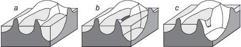
Figure 1.27. a) Flooding from all minima. b) The watershed line is the line where adjacent lakes meet. c) A catchment basin without a source is flooded through a neighboring basin

Throughout the book, we will come across such back and forth movements between node- and edge-weighted graphs.

1.8. Conclusion

Weighted graphs modeling has several advantages. The results are independent of the particular grid on which the images are represented and are valid whatever the dimension of the space one is working on. The same approach may be used for still or moving images, in two, three or more dimensions. Furthermore, graphs are able to model anything and everything. Node-weighted graphs may represent many structures other than images, and the tools developed for analyzing images may be used in much different contexts.

Upon completion of this survey on flooding and the watershed, we hope: we have successfully convinced readers that both concepts are useful in image processing and beyond; and, encouraged the study of the following mathematical developments, which will undoubtedly be useful for individual applications.