3
Mathematical Notions

3.1. Summary of the chapter

This chapter only covers the mathematical notions needed to understand the book content. For a comprehensive presentation of the algebraic foundations of Morphology, see chapter 2 written by Christian Ronse and Jean Serra in an excellent book on Mathematical Morphology [NAJ 13]

This chapter introduces the mathematical notions that are necessary for understanding the content of this book. These notions are not at all difficult; they belong to the algebraic theory of lattices and may not be familiar to some readers. They also constitute the algebraic basis of mathematical morphology, in particular the Galois adjunction from which erosions, dilations, openings and closings are derived. In conclusion, it sets the stage for the mathematical developments to follow.

3.2. Complete lattices

Given a set E, we define Ƥ (E) as the set of all its subsets: Ƥ (E) = {A|A ⊆ E}.

The classical operators of set theory ∪ and ∩ apply to Ƥ (E). The inclusion ⊂ relation between sets defines an order relation on Ƥ (E).

3.2.1. Partial order and partially ordered sets

A partial order relation is a binary relation, written ≤ over a set E satisfying the following axioms. For a, b, c ∈ E:

reflexivity: a ≤ a;

antisymmetry: if a ≤ b and b ≤ a, then a = b;

transitivity: if a ≤ b and b ≤ c, then a ≤ c.

For a, b ∈ E, if a ≤ b or b ≤ a, then a and b are comparable. Otherwise, they are incomparable. A partial order under which every pair of elements is comparable is called a total order. For instance, the set of integers constitutes a totally ordered set, as any pair of integers is comparable.

A set E with a partial order is called a partially ordered set or poset

3.2.2. Upper and lower bounds

For A ∈ Ƥ (E), an element x ∈ E is an upper bound of A if a ≤ x, for each element a in A.

For A ∈ Ƥ (E), an element x ∈ E is a lower bound of A if x ≤ a, for each element a in A.

REMARK 3.1.– An upper bound (respectively lower bound) of a subset A of Ƥ (E) does not necessarily belong to A.

3.2.3. Complete lattices

If the set Ā or upper bounds of A possesses a smallest element belonging to E, this element is called the least upper bound or supremum of A. We write ∨ A.

Similarly, if the set or lower bounds of A possesses a greatest element belonging to E, this element is called the greatest lower bound or infimum of A. We write ∧ A.

DEFINITION 3.1.– A partially ordered set E is called a complete lattice if every subset A of E has a supremum and an infimum in E.

Taking A = E shows that every complete lattice E has a greatest element or maximum and a least element or minimum. We write ω for the maximum and o for the minimum.

REMARK 3.2.– The set Ā or upper bounds of A is never empty as it contains at least ω and the supremum of A. Similarly, the set of lower bounds is never empty as it contains at least o and the infimum of A.

LEMMA 3.1.– A subset A does not necessarily possess a greatest element belonging to A. However, if this is the case and a ∈ A is this greatest element, then a is also the supremum of A.

PROOF.– a is itself an upper bound of A as a ≤ a. Being the greatest element of A, it is necessarily the supremum of A.

□

3.2.4. Dyadic relations on a complete lattice

As each element A of Ƥ (E) possesses an infimum ∧A and a supremum ∨A, we define for A, B ∈ Ƥ (E) : A ∨ B = ∨ (A ∪ B) and A ∧ B = ∧ (A ∪ B).

For a, b ∈ E: a ∨ b = ∨ (a, b) and a ∧ b = ∧(a, b), where (a, b) is the subset of E containing a and b.

We remark that A, B, A ∪ B, (a, b) are the elements of Ƥ (E), whereas A ∨ B = ∨ (A ∪ B), A ∧ B = ∧ (A ∪ B), a ∨ b = ∨ (a, b) and a ∧ b = ∧ (a, b) are the elements of E.

3.2.4.1. Properties

LEMMA 3.2.– For A, B ∈ Ƥ (E) : A ∨ B = ∨ (A ∪ B) = ∨ (∨A, ∨B) = (∨A) ∨ (∨B) and A ∧ B = ∧(A ∪ B) = ∧(∧A, ∧B) = (∧A) ∧ (∧B), where (∨A), (∨B), (∧A), (∧B) ∈ E.

PROOF.– Let us show that ∨ (A ∪ B) = ∨(∨A, ∨B) = (∨A) ∨ (∨B)

□

1) A ⊂ A ∪ B ⇒ ∪ ∨A < ∨ (A ∪ B). Similarly, ∨B < ∨ (A ∪ B).
∨ (A ∪ B) is an upper bound of ∨A and ∨B, which is larger than or equal to their least upper bound ∨(∨A, ∨B) : ∨(A ∪ B) > ∨ (∨A, ∨B).
2) ∨(∨A, ∨B) is the least upper bound of ∨A and ∨B, which is also an upper bound of A and B : it is larger than or equal to the least upper bound of A ∪ B : ∨ (A ∪ B) < ∪ (∨A, ∨B).
3) By antisymmetry, we deduce from both inequalities: ∨ (A ∪ B) = ∨ (∨A, ∨B).

3.3. Operators between complete lattices

3.3.1. Definition of an operator

For the sake of generality, we consider two complete lattices with distinct elements and order relations:

– a lattice V with an order relation written as≺, associated with an infimum ⋏ and a supremum ⋎;
– a lattice W with an order relation written as <, associated with an infimum ∧ and a supremum ∨.

We now define operators between the lattices. They are mappings associating with each element of a lattice an element of the other lattice:

– an operator α : V ↦ W associates with each x ∈ V the element α(x) ∈ W;
– an operator β : W ↦ V associates with each s ∈ W the element β(s) ∈ V.

These operators can be concatenated:

– the operator αβ associates with s ∈ W the element αβ(s) ∈ W;
– the operator βα associates with t ∈ V the element βα(t) ∈ V.

3.3.2. Properties of the operators

An operator α : V ↦ W increases if: x, y ∈ V: x ≺ y ⇒ α(x) < α(y).

An operator α : V ↦ W increases if: x, y ∈ V: x ≺ y ⇒ α(x) > α(y).

For operators for which the source and destination belong to the same lattice, we also define the following properties:

an operator ζ : V ↦ V is idempotent if ζζ = ζ;

an operator ζ : V ↦ V is anti-extensive if ζ(x) ≺ x;

an operator ζ : V ↦ V is extensive if x ≺ ζ(x);

an operator ζ : V ↦ V is an involution if ζζ = identity = Id_V.

A decreasing involution C : V ↦ V is called complementation.

3.3.3. Erosion and dilation

Two operators α and β commute if αβ = βα.

An operator α : V ↦ W commutes with the supremum if for x, y ∈ V : α(x ⋎ y) = α(x) ∨ α(y).

An operator α : V ↦ W commutes with the infimum if for x, y ∈ V : α(x ⋏ y) = α(x) ∧ α(y).

An increasing operator that commutes with the supremum is called a dilation.

A decreasing operator that commutes with the infimum is called an erosion.

3.3.4. Opening and closing

An increasing, idempotent and anti-extensive operator is called an opening.

An increasing, idempotent and extensive operator is called a closing.

3.4. The adjunction: a cornerstone of mathematical morphology

3.4.1. Adjoint erosions and dilations

DEFINITION 3.2.– The operators α : V ↦ W and β : W ↦ V form an adjunction if for υ ∈ V, ω ∈ W : α(υ) < ω ⇔ υ ≺ β(ω).

THEOREM 3.1.– If (α, β) form an adjunction, then α is a dilation and β is an erosion.

PROOF.– We suppose that (α, β) form an adjunction. Then, given s ∈ V and (t_i)_i∈I a family of elements of W : s ≺ β⋏ (t_i)_i∈I ⇔ αs < ⋏ (t_i)_i∈I ⇔ ∀i ∈ I : αs < t_i ⇔ ∀i ∈ I : s ≺ βt_i ⇔ s ≺ ⋏ (βt_i)_i∈I.

As ≺ is reflexive, we have s ≺ β⋏ (t_i)_i∈I. Replacing s by ⋏(βt_i)_i∈I in the preceding equivalences and reading from right to left: ⋏ (βt_i)_i∈I ≺ β⋏(t_i)_i∈I.

Similarly, replacing s by β⋏(t_i)_i∈I and reading from left to right: β⋏(t_i)_i∈I ≺ ⋏(βt_i)_i∈I.

As ≺ is antisymmetric, we obtain: ⋏ (βt_i)_i∈I = β⋏(t_i)_i∈I.

□

3.4.2. Increasingness

LEMMA 3.3.– If (α, β) form an adjunction, they are increasing operators

For u, v ∈ W, u < υ : β(u) = β(u ∧ v) = β(u) ⋏ β(v) ≺ β(v). For s, t ∈ V, s ≺ t : α(t) = α(s⋎t) = α(s) ∨ α(t) > α(s).

3.4.3. Unicity

If both β₁ and β₂ are adjunct operators of the same operator α, then β₁ = β₂. Indeed, for s, t ∈ V : s ≺ β₁t ⇔ αs < t ⇔ s ≺ β₂t. Replacing s by β₁t in the left inequality, we obtain: β₁t ≺ β₁t ⇔ β₁t ≺ β₂t. Replacing s by β₂t in the right inequality, we obtain: β₂t ≺ β₁t ⇔ β₂t ≺ β₂t. Thus, by antisymmetry of ≺: β₂t = β₁t.

3.4.4. Composition

If (α₁, β₁) and (α₂, β₂) form two adjunctions:

α₁, β₂ : V ↦ W and α₂, β₁ : W ↦ V

then (α₁α₂, β₂β₁ : W ↦ W) forms an adjunction.

Indeed, for υ, ω ∈ W : υ, ω ∈ W : α₁α₂υ < ω ⇔ α₂υ < β₁ω ⇒ υ < β₂ β₁ω.

3.4.5. Dual operators

We consider two complementation operators, i.e. decreasing involutions on V and W :

To each operator α : V ↦ W corresponds the dual operator: C_WαC_V : V ↦ W.

Similarly, to β : W ↦ V corresponds the dual operator: C_V βC_W : W ↦ V.

If (α, β) form an adjunction, then (C_vβC_w, C_wαC_v) also form an adjunction, where the operator C_vβC_w : W ↦ V is the dilation and the operator C_wαC_v is the erosion.

3.5. Openings and closings

3.5.1. Definitions

THEOREM 3.2.– If α : V ↦ W and β : W ↦ V form an adjunction, then the operator γ = αβ : W ↦ W is an opening and φ = βα : V ↦ V is a closing.

Let us show that the operator βα is indeed a closing, i.e. an increasing, extensive and idempotent operator. Similarly, the operator αβ is an increasing, anti-extensive and idempotent operator.

PROOF.– a) Product of two increasing operators, showing that βα is an extensive operator. Moreover, αβυ ≺ υ ⇐ βυ < βυ shows that αβ is an anti-extensive operator.

b) αβ being anti-extensive: αβυ ≺ υ ⇒ αβαυ < αυ and βα being extensive υ ≺ βαυ ⇒ αυ < αβαυ. By antisymmetry, we obtain: αυ = αβαυ. Applying β on both sides yields βαυ = βαβαυ, which shows that the closing is idempotent. The idempotence of the opening may be proved similarly and derives from the fact that βω = βαβω.

□

3.5.2. Elements with the same erosion or the same dilation

The preceding proof has established that αυ = αβαυ and βω = βαβω.

If s ∈ W verifies αβω < s < w, then by applying β on both sides of these inequalities: βαβω < βs < βω and since βω = βαβω, we obtain by anti-symmetry

βs = βω.

In fact, αβω is the smallest element of W that produces the same erosion as w:

Indeed: ⋀ {s | βω = βs} = ⋀ {s | βω < βs} = ⋀ {s | αβω < s} = αβω.

This shows that the erosion has no inverse element, since all elements verifying αβω < s < w produce the same erosion, with αβω being the smallest element of the family. This family has in general no greatest element.

Similarly, we show that βαυ is the largest element of V producing the same dilation as V : αυ = αβαυ.

3.5.3. The invariants of an opening or a closing

An element t is an invariant of an operator ψ if ψt = t. We denote the family of invariants of ψ by Inv (ψ).

We now study the family of invariants Inv(γ) ⊂ W and Inv(φ) ⊂ V of γ and φ.

LEMMA 3.4.– The family Inv(γ) of invariants of the opening γ is closed by the supremum ⋎. The family Inv(φ) of invariants of the closing φ is closed by the infimum ∧.

PROOF.– Consider two elements u, υ ∈ V that are invariant by the opening γ: γ(u) = u and γ(υ) = υ. Then, γ(u ⋎ υ) < u ⋎ υ = γ(u)⋎γ(υ) by anti-extensivity. Moreover, γ(u ⋎ υ) < u ⋎ υ = γ(u)⋎γ(υ) as γ is increasing.

□

For u ∈ V : αu ∈ Inv(γ) as αu = αβαu = (αβ)αu. Similarly, for υ ∈ W : βυ ∈ Inv(φ) as βυ = βαβυ = (βα)βv.

3.6. Complete lattices of functions

3.6.1. Definitions

We now consider a complete lattice Ƭ provided with a total order relation <. If Ɗ is an arbitrary set, we define Fun (Ɗ, Ƭ), the family of functions defined on the domain Ɗ and taking their value in Ƭ. A function f ∈ Fun(Ɗ, Ƭ) maps each element p ∈ Ɗ onto an element f(p) ∈ Ƭ.

The complete order relation < of Ƭ induces on Fun (Ɗ, Ƭ) the structure of a complete lattice with an induced order relation ≺:

If f and g are two functions of Fun(Ɗ, Ƭ), we define f ≺ g (order relation in Fun(Ɗ, Ƭ)) ⇔

∀p ∈ Ɗ: f(p) < g(p) (order relation in Ƭ).

In contrast to the order relation <, the order relation ≺ is not a total order, as not all the functions of Fun(Ɗ, Ƭ) are comparable.

3.6.2. Infimum and supremum

For a family of functions (f_i)i∈I of Fun(Ɗ, Ƭ) and s ∈ Ɗ:

the infimum is defined by 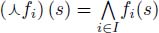and the supremum by .