4
Weighted Graphs

4.1. Summary of the chapter

This chapter sets the stage as it introduces graphs, collections of nodes or vertices linked by undirected edges or directed arcs. We will discuss two types of graphs: node-weighted graphs and edge-weighted graphs. Graphs are simple and abstract structures that are able to model all kinds of relations.

Node-weighted graphs may be used for modeling a topographic surface: the nodes represent positions in a domain. An edge between two nodes simply indicates that the corresponding positions are neighbors. The weights of the nodes express the altitude of the surface at the corresponding locations.

Edge-weighted graphs may be used for modeling the relations between the catchment zones of a topographic surface. Each catchment zone is represented by a node. Two catchment zones separated by a pass point are linked by a weighted edge, with the edge weight being the altitude of the pass point.

This interpretation of node- or edge-weighted graphs will be inspiring for operators which make sense when applied to a topographic surface. However, the same operators may take other interpretations if the graphs model other structures than topographic surfaces.

A path is a series of nodes such that two successive nodes are linked by an edge. The weights of the nodes or edges enable us to define flowing paths, followed by a drop of water deposited on a node. On a node-weighted graph, a drop of water may move from node p to node q, if the weight of q is not higher than the weight of p, as a drop of water never moves upwards. On an edge-weighted graph, there is no relative altitudes between nodes. A drop of water deposited on a node p quits this node through the lowest adjacent edge.

The remaining topographic concepts derive from these simple elementary motions of a drop of water between adjacent nodes.

In this chapter, we separately study the particular form taken by these topographical concepts for node-weighted and edge-weighted graphs. There are many similarities between the two types of graphs:

• – Two nodes belong to a flat zone if they are linked by a path along which a drop of water may glide in both directions.
• – A flat zone from where a drop of water cannot escape is a regional minimum.
• – All nodes linked with a regional minimum by a flowing path constitute the catchment zone of this minimum.

There are also some significant differences between the two types of graphs:

• – Some nodes in a node-weighted graph are surrounded by nodes with a higher weight. Such nodes are isolated regional minima nodes. Isolated regional minima nodes do not exist in edge-weighted graphs, as each node has at least one adjacent edge (we suppose that the graph is connected, each node being connected with at least one other node). A regional minimum in an edge-weighted graph contains at least two nodes, linked by an edge, the lowest adjacent edge for both of them.
• – In a node-weighted graph, each edge is a flowing edge for its extremity holding the highest weight. If both extremities have the same weight, it is a flowing edge of both extremities. In an edge-weighted graph, on the contrary, there may exist edges which are not the lowest adjacent edge of one of their extremities. Such edges are never crossed by a drop of water deposited at one of their extremities, as this drop of water will follow an edge with a lower weight.

4.2. Reminders on graphs

4.2.1. Directed and undirected graphs

4.2.1.1. Definitions

A graph G = [, ε] contains a set of vertices or nodes and a set ε of edges; an edge being an unordered pair of vertices. The nodes are designated with small letters: p, q, r... The edge linking the nodes p and q is denoted by e_pq or by (p – q).

A directed graph, also called a digraph , contains a set of vertices or nodes and a set of arcs, an arc being an ordered pair of vertices.

Undirected edges are simply called edges, whereas directed edges are called arcs. If p and q are neighboring nodes, then (p – q) denotes an undirected edge, whereas (p → q) or (q → p) denotes directed arcs (also called arrows). If both arcs (p → q) and (q → p) exist, we write (p ↔ q) or (p ⇆ q) that consists of a bidirectional arrow.

4.2.1.2. Subgraphs and partial graphs

4.2.1.2.1. Subgraphs

For an undirected graph, the subgraph spanning a set A ⊂ is the graph G_A = [A, ε_A], where ε_A are the edges linking two nodes of A: ε_A = {(p – q) ∈ ε | p, q ∈ A}.

For a directed graph , the subgraph spanning a set A ⊂ is the graph , where _A are the arcs of connecting two nodes of A : or (q → p) or .

4.2.1.2.2. Partial graphs

The partial graph is associated with a subset of edges. Its nodes are all nodes of whose extremities are linked by an edge of , where .

The partial digraph is associated with a subset of arcs. Its nodes are all nodes of whose extremities are linked by an arc of , where or (q → p) or .

4.2.1.3. Paths and cycles

4.2.1.3.1. Undirected graphs G

A path, π, is a sequence of vertices and edges, interweaved in the following way: π starts with a vertex, say p, followed by an edge (p – q), incident to p, followed by the other endpoint q of e_pq, and so on.

• We will use various notations:
• : an undirected path from p to q.
• : an undirected path of origin p.
• |π_pq|: number of edges of the path π_pq.
• : concatenation of two paths.

4.2.1.3.2. Directed graphs

A directed path, , is a sequence of vertices and arrows, interweaved in the following way: π starts with a vertex, say p, followed by an arrow (p → q) with origin p, followed by the arrowhead q of (p → q), and so on.

• : a directed path from p to q.
• : a bidirectional path between p and q.
• : a directed path starting at p.
• : number of edges of the path .
• : concatenation of two directed paths.

4.2.1.4. Cocycles and neighborhoods

4.2.1.4.1. Undirected graphs G

A cycle is a path whose origin and extremity coincide.

The cocycle of a set Y is the set of all edges with one extremity in a subset Y of the nodes and the other in the complementary set Ȳ:

4.2.1.4.2. Directed graphs

The cocycle of a set Y is the set of all arrows with one extremity in a subset Y of the nodes and the other in the complementary set Ȳ:

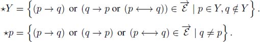
We may distinguish between the outgoing cocycles where all arrows have their origin in Y and the incoming cocycles where all arrows have their arrowheads in Y.

4.3. Weight distributions on the nodes or edges of a graph

Edges and/or nodes may be weighted with weights taken in a totally ordered set Ƭ. We define two families of functions:

• : the functions defined on the nodes for a value of Ƭ.
• : the functions defined on the edges ε for a value of Ƭ.

The function takes the value η_pq on the edge e_pq of the graph G or on the arc in ; the function takes the weight ν_p on the node p in G and .

Nodes and edges may hold weights or not. We will distinguish:

• – G(ν, η): a node- and edge-weighted graph.
• – G(ν, nil): a node-weighted graph, with unweighted edges.
• – G(nil, η): an edge-weighted graph, with unweighted nodes.
• – G(nil, nil): an unweighted graph.

4.3.1. Duality

The first operator C is a decreasing involution or complementation. According to T, it takes the following two forms:

If T represents signed numbers, Cν = –ν for and Cη = –η for .

If T = [0, K], then Cν = K – ν for and Cη = K – η for .

To each operator , we assign a dual operator: . And for an operator .

4.3.2. Erosions and dilations, openings, closings

4.3.2.1. Erosions and dilations between node and edge weights

DEFINITION 4.1.– We define two operators between edge weights η and node weights ν:

• – an erosion [ε_en ν]_ij = ν_i ∧ ν_j and its adjoint dilation ;
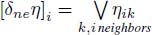• – a dilation [δ_en ν]_ij = ν_i ∨ ν_j and its adjoint erosion .

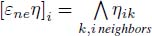LEMMA 4.1.– The four operators are two-by-two dual or adjoint operators.

• – ε_ne and δ_en are adjunct operators.
• – ε_en and δ_ne are adjunct operators.
• – ε_ne and δ_ne are dual operators.
• – ε_en and δ_en are dual operators.

PROOF.– Adjunction: Consider, for the same graph, an arbitrary function on the nodes and an arbitrary function on the edges. Then, . Duality: [ε_en(–ν)]_ij = –ν_i ∧ –ν_j = –(ν_i ∨ ν_j) = –[δ_en ν]_ij. Thus, δ_en ν = – [ε_en(–ν)].

□

4.3.2.2. Composition of operators

By composition, we obtain the following operators:

• – an erosion from node to node: ε_N = ε_neε_en;
• – a dilation from node to node: δ_N = δ_neδ_en;
• – an opening from node to node: γ_n = δ_neε_en;
• – a closing from node to node: φ_n = ε_neδ_en.

By composition, we obtain the following operators:

• – an erosion from edge to edge: ε_E = ε_enε_ne;
• – a dilation from edge to edge: δ_E = δ_enδ_ne;
• – an opening from edge to edge: γ_e = δ_enε_ne;
• – a closing from edge to edge: φ_e = ε_enδ_ne.

4.3.2.3. Gradient operators

As the functions ν, η and the functions produced by one of the above operators take all their values in T, a lattice on numbers, on which a subtraction exists, we may combine dilations and erosions to form gradient operators. These operators, first defined by Serge Beucher, are obtained by subtracting an erosion from a dilation. We may thus define Beucher Gradient operators:

• – assigns to each edge the difference between the highest weight of its extremities and the lowest.
• – assigns to each node the difference between the highest weight in its neighborhood and the lowest.
• – assigns to each node the difference between the highest weight of its adjacent edges and the lowest.
• – assigns to each edge the difference between the highest weight in its neighborhood and the lowest.

4.3.2.4. The special role of the flowing adjunction: (δ_en, ε_ne)

In the context of the watershed and flooding theory, we will mostly use the flowing adjunction: (δ_en, ε_ne) and the derived opening γ_e and closing φ_n. They nicely reveal the intrication of the node or edge weights with the graph structure itself.

For instance, if a node-weighted graph has no isolated regional minima, i.e. node with only higher neighbors, then the node weight function υ is invariant by the closing φ_n. On the contrary, if such nodes exist, their weight is increased by the closing φ_n as is illustrated in Figure 4.1. Figure 4.1 successively presents a node-weighted graph G(ν, nil), followed by the edge-weighted graph G(nil, δ_enν) and finally by G(φ_nν, nil). There is a node in the upper part of the graph with weight 1 which is an isolated regional minimum. The weight of this node is increased in the graph G(φ_nν, nil), whereas in all the other nodes, their weights are unchanged.

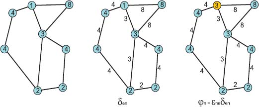
Figure 4.1. From left to right, a node-weighted graph G(ν, nil), the edge-weighted graph G(nil, δ_enν) and the node-weighted graph G(φ_nν, nil). The orange node on the right has its weight changed between G(ν, nil) and G(φ_nν, nil). For a color version of the figures in this chapter, see www.iste.co.uk/meyer/topographical1.zip

Similarly, if in an edge-weighted graph, each edge is the lowest adjacent edge of one of its neighbors, then the edge weight function is invariant by the opening γ_e. If this is not the case, the weight of such edges is lowered by the opening γ_e, as shown in Figure 4.2. Figure 4.2 presents an edge-weighted graph G(nil, η), followed by the node-weighted graph G(ε_neη, nil) and on the right the graph G(nil, γ_eη). The edge G(nil, γ_eη) whose weight has been lowered is highlighted by a red color. These edges are not the lowest edges of their extremities.

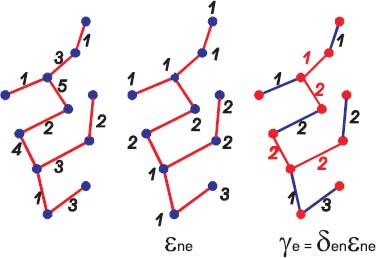
Figure 4.2. From right to left, an edge-weighted graph G(nil, η), the node-weighted graph G(ε_neη, nil) and on the right the graph G(nil, γ_eη). The red edges in the graph G(nil, γ_eη) have their weights lowered between the graphs G(nil, η) and the graph G(nil, γ_eη). These edges are not the lowest edges of one of their extremities

4.3.3. Labels

It will also be useful to attribute labels to the nodes. Typically, such labels serve to encode the various sub-structures extracted from the graph, for instance, for labeling the equivalence classes associated with equivalence relations defined on a graph. All nodes belonging to the same equivalence class share the same label. Serving for numbering and identifying structures, the labels are generally integers. Thus, the label function ϖ belongs to , the functions defined on the nodes for a value of ℕ.

4.4. Exploring the topography of graphs by following a drop of water

A topographic surface may be explored by following a drop of water deposited on its surface. By analogy, we will analyze and compare the “topography” of both edge-weighted or node-weighted graphs. This topography will be described by analyzing the trajectories followed by a drop of water moving from node to node.

For both types of graphs, node-weighted and edge-weighted, we define the elementary motions, a drop of water may follow from a node to the next one. An edge (p, q) is a flowing edge of a node p if a drop of water deposited at p is able to move to the node q.

Concatenating the flowing edges produces flowing paths. The flowing paths, in turn, serve to define regional minima, which are zones impossible to leave by following a flowing path. All nodes linked with a regional minimum by a flowing path form the catchment zone of this regional minimum.

We now precisely define the flowing edges, followed by a drop of water from node to node, highlighting the similarities and differences between the topographies of node-weighted and edge-weighted graphs.

4.5. Node-weighted graphs

We consider a node-weighted graph G(ν, nil).

4.5.1. Flat zones and regional minima

We define a binary relation between neighboring nodes: p * q ⇔ ν_p = ν_q.

This relation is reflexive and symmetrical. Its transitive closure constitutes an equivalence relation . For p ≠ s, the relation p s holds if a path linking p and s exists, whose nodes have the same weight. As the relation is also symmetrical and reflexive, it is an equivalence relation.

DEFINITION 4.2.– The equivalence classes of ps are the flat zones of the graph.

DEFINITION 4.3.– A regional minimum of G(ν, nil) is a flat zone without lower neighboring nodes.

REMARK 4.3.– A node without a neighboring node with the same weight or a lower weight is an isolated regional minimum.

4.5.2. Flowing paths and catchment zones

A drop of water may quit a node p, follow an edge e_pq and reach the node q iff the nodes p and q verify ν_p ≥ ν_q. This means that a drop of water never moves upwards.

DEFINITION 4.4.– The edge e_pq is a flowing edge of its extremity p iff ν_p ≥ ν_q.

Each edge of a node-weighted graph is a flowing edge of one of its extremities. Take the edge e_st, for instance. The edge e_st is a flowing edge of s if ν_s ≥ ν_t or of t if ν_t ≥ ν_s. If ν_t = ν_s, then e_st is a flowing edge of both its extremities.

DEFINITION 4.5.– A path p – e_pq – q – e_qs – s… is a flowing path if each node except the last one is followed by one of its flowing edges.

It follows that the weights along a flowing path are never increasing: if p, q, s are three successive nodes on a flowing path, then ν_p ≥ ν_q ≥ ν_s.

LEMMA 4.2.– Any node outside a regional minimum is the first node of at least a flowing path leading to a regional minimum.

PROOF.– Take an arbitrary node p not belonging to a regional minimum. The node p has at least a neighboring node q which is lower or equal. If ν_q < ν_p, then p – e_pq – q is the beginning of a flowing path. If q itself does not already belong to a regional minimum, the reasoning applied to p may now be applied to the node q. If ν_q = ν_p, then p and q belong to a flat zone X which is not a regional minimum. X has a neighboring node with a lower weight: a pair of nodes s and t, exist s ∈ X, , verifying ν_s > ν_t. As X is a flat zone, a path π linking p and t exists inside X along which all nodes have the same weight. Concatenating the path π with the edge e_st produces a flowing path linking the node p with a lower node t. The same reasoning is then applied to the node s.

Thus, we construct a flowing path of origin p. Each step takes as input a flowing path ending with a node t_k, and expands it into a new flowing path with a node t_k+1 with a lower weight than t_k. As the weights from t_k to t_k+1 are strictly decreasing, each step introduces at least one new node, never met before, into the flowing path. Since the number of nodes of the graph is finite, the process necessarily finishes inside a flat zone without lower neighbors, i.e. a regional minimum.

□

As any node is linked with at least one regional minimum, we may now define the catchment zone of a regional minimum.

DEFINITION 4.6.– The catchment zone of a regional minimum m is the set of nodes which are linked with a node inside m by a flowing path.

It results from the previous analysis that each node belongs to at least one catchment zone. It may, however, be linked by two flowing paths with two distinct regional minima, and thus belongs to two catchment zones, which overlap. Methods are presented in the following chapters for reducing the overlapping between catchment zones.

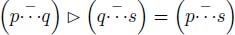
REMARK 4.4.– In the previous section, we defined p*q ⇔ ν_p = ν_q. This relation p*q may also be expressed using the flowing edges. For p ≠ q, we say that iff the edge e_pq is a flowing edge of both p and q. Indeed, ν_p = ν_q implies that e_pq is a flowing edge of p and of q. Inversely, if e_pq is a flowing edge of p, we have ν_p ≥ ν_q, and simultaneously, if it is a flowing edge of q, we have ν_q ≥ ν_p; both relations yielding ν_p = ν_q. In the case of node-weighted graphs, the relation p*q and are thus equivalent. The relation , however, is more general, as it may be associated with each definition of flowing edges. In the next section, we meet flowing edges defined on edge-weighted graphs. In the next chapter, we meet flowing edges on unweighted-directed graphs. In this case, the relation holds if and only if (p ⇆ q).

REMARK 4.5.– This remark will be useful in the next chapter, in which we replace the flowing edges with directed arcs and study the topography of unweighted digraphs.

4.6. Edge-weighted graphs

We now consider an edge-weighted graph G(nil, η) and analyze the trajectories that a drop of water may follow on such a graph.

4.6.1. Flat zones and regional minima

We say that two edges are adjacent if they share a common extremity, as, for instance, the edges e_pq and e_qr. We define a symmetrical relation between adjacent edges: e_pq ~ e_qr ⇔ η_pq = η_qr.

This relation is reflexive (e_pq ~ e_pq) and symmetrical (e_pq ~ e_qr ⇒ e_qr ~ e_pq). Its transitive closure ≈ constitutes an equivalence relation between edges. The relation e_pq ≈ e_st holds if a path linking p and t exists along which all edges have the same weight.

DEFINITION 4.7.– The equivalence classes of the equivalence relation ≈ are the edge flat zones of the edge-weighted graph.

REMARK 4.6.– As equivalence classes of an equivalence relation are the edge flat zones disjoint. More precisely, they are “edge disjoint”, two such flat zones have no edge in common. However, they may have nodes in common. A node p may have two adjacent edges e_pq and e_ps with distinct weights, each of them belonging to a different edge flat zone.

DEFINITION 4.8.– A regional minimum of G(nil, η) is an edge flat zone without an adjacent edge with a lower weight.

4.6.2. Flowing paths and catchment zones

A drop of water at a node p compares the weights of all edges to quit p, and follows one of the adjacent edges with the lowest weight.

DEFINITION 4.9.– An edge (p, q) is a flowing edge of the node p, if it is one of the lowest adjacent edges of p

In contrast to node-weighted graphs, in an edge-weighted graph, there may exist edges which are not flowing edges. Consider an edge e_st with a weight λ. If the nodes s and t have adjacent edges with lower weights than λ, then e_st is not a flowing edge. A drop of water deposited at s or t will never follow the edge e_st.

DEFINITION 4.10.– A path p – e_pq – q – e_qs – s… is a flowing path if each node except the last one is followed by one of its flowing edges.

It follows that the weights of the successive edges in a flowing path are never increasing (if p, q and r are three successive nodes of a flowing path, then e_qr is one of the lowest edges of q and thus e_pq ≥ e_qr).

LEMMA 4.3.– Any node outside a regional minimum is the first node of a flowing path leading to a regional minimum.

PROOF.– Take an arbitrary node p not belonging to a regional minimum. Consider one of the edges with minimum weight linking this node with a node q. The path p – e_pq – q is a flowing path. If q belongs to a regional minimum, the lemma is verified. If not, we expand this path until reaching a regional minimum. We apply the same method to q and get the third node s and a path p – e_pq – q – e_qs – s which is a flowing path. Again, if qs belongs to a regional minimum, the lemma is verified. If not and if η_qs < η_pq, the altitude of the path has decreased and we repeat the same process until a regional minimum is reached, which, as we will establish below, cannot fail to happen. If η_qs = η_pq, then p, q and s belong to a flat zone X which is not a regional minimum. If the internal edges of X have a weight equal to λ, and since X is not a regional minimum, X has an edge in its cocycle with a weight lower than λ: a pair of nodes r and t, exist r ∈ X, , verifying η_rt < λ. As X is a flat zone, a path π linking p and t exists inside X along which all edges have the same altitude. Concatenating the path π with the edge e_rt is a flowing path linking the node p with r, the last edge e_rt of this path having decreased. The same process is then applied to the node r and repeated. Ultimately, this process reaches a regional minimum. Indeed, both processing steps we just described construct a flowing path of origin p. Each step takes as input a flowing path and expands it into a new flowing one with a lower extremity. As the weights of these last edges are strictly decreasing, each step introduces at least one new edge, never met before, into the flowing path. Since the number of edges of the graph is finite, the process necessarily finishes inside a flat zone without a lower edge in its cocycle, i.e. a regional minimum.

□

As any node is linked with at least one regional minimum, we may now define the catchment zone of a node.

DEFINITION 4.11.– The catchment zone of a regional minimum m is the set of nodes which are linked with a node inside m by a flowing path.

It results from this analysis that each node belongs to at least one catchment zone. However, the same node may be linked by two flowing paths with two distinct regional minima, and thus belongs to two distinct catchment zones, which overlap. Later, we present methods for reducing the zones where catchment zones overlap, without modifying the initial edge or node weights. Instead, we edit the graph in order to reduce the number of flowing paths.

4.6.3. Even zones and regional minima

The second symmetrical relation, may be defined, this time between neighboring nodes. The relation is verified between the nodes p and q if the edge e_pq connecting them is a flowing edge for both. In other terms, e_pq is one of the lowest adjacent edges of p and of q : .

REMARK 4.7.– We already met this same binary relation in the preceding section treating of node-weighted graphs, for which e_pq is a flowing edge of both its extremities p and q if and only if ν_p = ν_q.

We associate with the relation: holding if a path linking p and s exists, such any two successive nodes u and υ on this path verify u υ. This relation is transitive: if and , by concatenating the paths π_ps and π_st along which the relation holds, we obtain a path π_pt along which also holds.

By convention, we consider the relation to be reflexive: . It is obviously symmetrical. It is thus an equivalence relation.

DEFINITION 4.12.– The equivalence classes of are called even zones of the edge-weighted graph.

If p, q, s verify p q and q s, then ; . It follows η_pq = η_qs.

The reverse implication is not true. If p, q, s are three nodes linked by edges whose weights verify η_pq = η_qs, it does not necessarily follow that p q and q s. Indeed, any of the nodes p, q, s may have an adjacent edge with a lower weight than η_pq = η_qs. If, for instance, p has a neighboring node t verifying η_pt < η_pq, then the relation p q is false.

PROPOSITION 4.1.– In a connected edge-weighted graph G(nil, η), an even zone impossible to quit by following a flowing path is a regional minimum of the graph.

PROOF.– We first remark that inside an even zone, all edges have the same weight. Suppose that a set of nodes X constitutes an even zone with weight λ, which is impossible to quit following a flowing edge. This means that if p ∈ X and e_pq is a flowing edge of origin p, then q also belongs to X and the edge e_qp is also the lowest edge of q. The edges of X constitute a flat zone of the graph without adjacent lower edges, i.e. a regional minimum of G(nil, η).

□

REMARK 4.8.– We now have two characterizations of regional minima in edge-weighted graphs. The first one as edge flat zones, without outgoing flowing paths, concerns only edges. The second one considers even zones and concerns the nodes linked by bidirectional paths. They both have in common that no flowing paths exist, which makes it possible to quit a regional minimum. The second definition, based on even zones, will be generalized later to unweighted digraphs.

4.7. Comparing the topography of node-weighted graphs and edge-weighted graphs

We have studied the topography of node-weighted graphs and edge-weighted graphs by considering the possible trajectories of a drop of water. We have considered all possible trajectories by excluding only trajectories where a drop of water moves upwards from a node to the next. An edge e_pq such that a drop of water may move from the node p to the node q is a flowing edge.

Flowing edges have been defined for both node- and edge-weighted graphs: the first is based on the node weights and the second is based on the edge weights. The flowing paths are then simply series of flowing edges, one flowing edge ending where the next starts. The major topographical structures of node- and edge-weighted graphs involve the paths.

• – All nodes linked with a node p by a path whose nodes have the same weight constitute a node flat zone in a node-weighted graph.
• – All nodes linked with a node p by a path whose edges have the same weight constitute an edge flat zone in an edge-weighted graph.
• – All nodes linked with a node p by a bidirectional flowing path constitute an even zone in an edge-weighted graph (an edge is a bidirectional flowing edge, if it is one of the lowest edges of each of its extremities).
• – A regional minimum is a flat zone which is impossible to quit by a flowing path.
• – The catchment zone of a regional minimum is the set of nodes linked by a flowing path with this regional minimum.
• – All nodes belong to at least one catchment zone.