5
Flowing Graphs

5.1. Summary of the chapter

We first explain how to assign weights to the nodes in an edge-weighted graph or to the edges in a node-weighted graph:

• – In a node-weighted graph G(ν, nil), each edge is the flowing edge of one of its extremities, whose weight may be assigned to the edge. The weight η_pq assigned to the edge e_pq is the result of a dilation between the node weights and the edge weights: δ_enν = ν_p ∨ ν_q. Thus, we obtain a node- and edge-weighted graph G(ν, δ_enν).
• – In an edge-weighted graph G(nil, η), each node p is the origin of one or several flowing edges, the adjacent edges with minimal weight. This weight may be assigned to the node p. It is the result of an erosion between the edge weights and the node weights . Thus, we obtain a node- and edge-weighted graph G(ε_neη, η).

As the graphs now have node and edge weights, we distinguish the n-flowing edges defined by only considering the node weights and the e-flowing edges defined by only considering the edge weights. The inclusion { n-flowing edges of G(ν, nil)} ⊂ { e-flowing edges of G(nil, δ_enν)} becomes an identity in the case where ν = ε_neδ_enν = φ_nν, a closing on the node weights ν. This condition is met for a node-weighted graph without isolated regional minima (IRM). Isolated regional minima may be suppressed by editing the graph and connecting each IRM with itself by a loop edge. We obtain an edited node-weighted graph ↻ G(ν, nil) in which the node weights verify ν = ε_neδ_enν = φ_nν. If we set η = δ_enν, we have ν = ε_neδ_enν = ε_neη.

Similarly, the inclusion {e-flowing edges of G(nil, η)} ⊂ {n-flowing edges of G(ε_neη, nil)} becomes an equality if η = δ_enε_neη = γ_eη, an opening on the edge weights η. An edge-weighted graph may contain edges which are not the lowest edge of one of their extremities. Such edges do not exist in a node-weighted graph. If we suppress such edges in G(nil, η), we obtain the pruned graph ↓ G(nil, η), in which the function η verifies η = δ_enε_neη = γ_eη. If we set ν = ε_neη, we have η = δ_enε_neη = δ_enν.

The augmented graph ↻ G(ν, δ_enν) and the pruned graph ↓ G(ε_neη, η) are called flowing graphs since their node weights ν and edge weights η verify ν = ε_neη and η = δ_enν. Their flowing edges, regional minima and catchment zones are identical whether we consider the node weights alone or the edge weights alone. In a flowing path, each node is followed by an edge of the same altitude.

This chapter illustrates these relationships by modeling node- and edge-weighted graph as a network of tanks interconnected by pipes. The level of water in the tanks represents the node weights and the altitude of the pipes represents the edge weights.

5.2. Towards a convergence between node- and edge-weighted graphs

Node- and edge-weighted graphs share several common but also distinguishing features associated with the flowing edges. We call the flowing edges of a node-weighted graph as n-flowing edges. In edge-weighted graphs, we speak of e-flowing edges. If the context is clear and there is no ambiguity, we simply use the word flowing edges.

This chapter aims to establish an equivalence between node- and edge-weighted graphs. We aim to associate each node (respectively edge) weighted graph with an edge (respectively node) weighted graph such that the regional minima and catchment zones of both graphs are identical.

5.2.1. The flowing edges in a node-weighted graph G(ν, nil)

5.2.1.1. e-Flowing graphs

The edge e_pq is an n-flowing edge of its extremity p, iff ν_p ≥ ν_q. Thus, a node only having neighbors with a higher weight is not the origin of a flowing edge, it is an isolated regional minimum.

On the contrary, for each edge e_pq, we have either ν_p ≥ ν_q or ν_q ≥ ν_p. Hence, each edge is a flowing edge of one of its extremity (or of both if ν_p = ν_q).

DEFINITION 5.1.– A graph in which each edge is the flowing edge of one of its extremities is called the e-flowing graph.

PROPOSITION 5.1.– A node-weighted graph G(ν, nil) is an e-flowing graph.

5.2.1.2. Assigning weights to the edges of a node-weighted graph G(ν, nil)

As each edge e_pq of a node-weighted graph is the flowing edge of one of its extremities, it may be assigned the weight of this extremity. This weight may be expressed by a unique expression, ν_p ν ν_q, covering all cases. Indeed, the edge e_pq may be the flowing edge of p, q or both p and q:

{e_pq n-flowing edge of p} ⇔ {ν_p ≥ ν_q} ⇔ {ν_p = ν_p ∨ ν_q} or

{e_pq n-flowing edge of q} ⇔ {ν_q ≥ ν_p} ⇔ {ν_q = ν_p ∨ ν_q} or

{e_pq n-flowing edge of p and q} ⇔ {ν_q = ν_p} ⇔ {ν_p = ν_q = ν_p ∨ ν_q}

Thus, whether e_pq is a flowing edge of p, q or of both its extremities, we may assign to e_pq a weight η_pq = ν_p ∨ ν_q, symmetrical in p and in q.

5.2.2. The flowing edges in an edge-weighted graph G(nil, η)

5.2.2.1. n-Flowing graphs

The edge e_pq is an e-flowing edge of its extremity p, iff e_pq is one of the edges adjacent to p with the smallest weight. If the graph is connected, it has no isolated nodes, and each node is the origin of one or several e-flowing edges.

On the contrary, edges which may exist that are not the e-flowing edge of one of their extremities.

DEFINITION 5.2.– A graph in which each node is the origin of a flowing edge is called the n-flowing graph.

Since each edge in a connected edge-weighted graph is the origin of at least one flowing edge, we have the following proposition:

PROPOSITION 5.2.– A connected edge-weighted graph is an n-flowing graph.

5.2.2.2. Assigning weights to the nodes of an edge-weighted graph G(nil, η)

As each node p is the origin of an e-flowing edge e_pq, it seems natural to assign to p the weight of this e-flowing edge: ν_p = η_pq. Let us compute this weight η_pq.

{e_pq e-flowing edge of p} ⇔ {η_pq ≤ η_ps for each neighboring node s of p} ⇔

As each node p in an edge-weighted graph is the origin of an e-flowing edge, it is assigned the weight of this edge. This weight is symmetrical with respect to all neighbors of p.

5.2.3. Flowing graphs

The major structural difference between node- and edge-weighted graphs is linked with their flowing edges:

• – In a node-weighted graph, each edge is the flowing edge of one of its extremities. Such a graph is called an e-flowing graph.
• – In an edge-weighted graph, each node is the origin of a flowing edge. Such a graph is called an n-flowing graph.

We will show the equivalence between the two types of graphs if we are able to construct graphs which are at the same time e-flowing and n-flowing graphs.

DEFINITION 5.3.– A flowing graph is a graph which is at the same time an e-flowing and an n-flowing graph.

In a flowing graph, each edge is the flowing edge of one of its extremities and each node is the origin of a flowing edge, establishing a kind of coupling between nodes and flowing edges.

5.3. The flowing adjunction

We have defined the following operators, which are able to assign weights to the nodes of edge-weighted graphs or to the edges of node-weighted graphs:

• – In a node-weighted graph, each edge is the n-flowing edge of one of its extremities and gets the weight of this extremity: η_pq = ν_p ∨ ν_q. This operator is a dilation between the node weights and the edge weights, which can be written as: (δ_enν)_pq = ν_p ∨ ν_q.
• – In an edge-weighted graph, each node is the origin of a flowing edge and gets the weight of this edge: . This operator is an erosion between the edge weights and the node weights, which can be written as: .

Both operators form an adjunction between the node and the edge weights. We call it the flowing adjunction.

THEOREM 5.1.– The pair of operators (δ_en, ε_ne) forms an adjunction: .

PROOF.– Consider, for the same graph, an arbitrary function on the nodes and an arbitrary function on the edges. Then:

□

As recalled in the primer on adjunction, if the couple (δ_en, ε_ne) forms an adjunction, then [SER 88]:

• – δ_en is a dilation from into ;
• – ε_ne is an erosion from into ;
• – γ_e = δ_enε_ne is an opening from into ;
• – φ_n = ε_neδ_en is a closing from into .

The flowing adjunction has already been used for studying watershed and waterfall algorithms in [MEY 09]. These operators belong to a larger family of operators between nodes, edges and faces of planar graphs (which are used to construct micro-viscous leveling and filters [MEY 07a] and binary filters [COU 09b]).

5.4. Flowing edges under closer scrutiny

5.4.1. Relations between the flowing edges of G(ν, nil) and G(nil, δ_enν)

In a node-weighted graph G(ν, nil), each edge is the n-flowing edge of one of its extremities and gets its weight, producing the edge-weighted graph G(nil, δ_enν). We now examine the relations of the flowing edges of G(ν, nil) and G(nil, δ_enν).

If e_pq is a flowing edge of p, we have η_pq = ν_p ∨ ν_q = ν_p ≤ ν_p ∨ ν_s = η_ps for each neighboring node s of p. Thus, e_pq is one of the adjacent edges of p with the smallest weight, i.e. an e-flowing edge of p in G(nil, δ_enν).

The inverse is not true. Take an isolated regional minimum m in G(ν, nil). All its neighboring nodes have a higher weight. If s is one of the neighbors of m with the lowest weight, then η_ms = ν_m ∨ ν_s ≤ ν_m ∨ ν_t = η_mt for each neighboring node t of p, showing that e_ms is an e-flowing edge of m in G(nil, δ_enν), but not in G(ν, nil).

We have thus established the following inclusion: {n-flowing edges of G(ν, nil)} ⊂ { e-flowing edges of G(nil, δ_enν)}. Note that this inclusion is strict in the presence of isolated regional minima.

5.4.2. Relations between the flowing edges of G(nil, η) and G(ε_neη, nil)

In an edge-weighted graph G(nil, η), each node is the origin of an e-flowing edge and gets the weight of this edge, producing a node-weighted graph G(ε_neη, nil). If e_pq is an e-flowing edge of p, we have ν_p = (ε_neη)_p = η_pq ≥ (ε_neη)q = νq, showing that the edge e_pq is also an n-flowing edge of p in the graph G(ε_neη, nil).

The inverse is not true. As G(ε_neη, nil) is an e-flowing graph, each of its edges is a flowing edge. The graph G(nil, η), on the contrary, may have edges which are not the lowest edge of one of their extremities. Such edges are nevertheless flowing edges in G(ε_neη, nil).

We have thus established the following inclusion: {e-flowing edges of G(nil, η} ⊂ { n-flowing edges of G(ε_neη, nil)}. This inclusion is strict if the graph G(nil, η) possesses edges which are not flowing edges, i.e. edges which are not the lowest neighboring edge of one of their extremities.

5.4.3. Chaining the inclusions between flowing edges

We have established the following inclusion rules for the flowing edges of node-or edge-weighted graphs:

1. 1) {n-flowing edges of G(ν, nil)} ⊂ {e-flowing edges of G(nil, δ_enν)};
2. 2) {e-flowing edges of G(nil, η)} ⊂ {n-flowing edges of G(ε_neη, nil)}.

By chaining both relations, we obtain new inclusions.

5.4.3.1. Node-weighted flowing graphs G(ν, nil)

We chain the inclusions 1 and 2: {n-flowing edges of G(ν, nil)} ⊂ {e-flowing edges of G(nil, δ_enν)} ⊂ {n-flowing edges of G(ε_neδ_enν, nil)}. A sufficient condition for the extremal terms to be identical is ν = ε_neδ_enν = φ_nν. In this case, the n-flowing edges of G(ν, nil) and the e-flowing edges of G(nil, δ_enν) are identical. As any node-weighted graph, the graph G(ν, nil) is an e-flowing graph, and as any edge-weighted graph, the graph G(nil, δ_enν) is an n-flowing graph. As they have the same flowing edges, both are an n-flowing graph and an e-flowing graph, i.e. a flowing graph.

COROLLARY 5.1.– A sufficient condition for a node-weighted graph G(ν, nil) to be a flowing graph is ν = φ_nν.

If we define η = δ_enν, we have ν = φ_nν = ε_neδ_enν = ε_neη.

LEMMA 5.1.– If ν = φ_nν, the adjunction (ε_ne, δ_en) produces a perfect coupling between the node and edge weights: η = δ_enν and ν = ε_neη.

5.4.3.2. Edge-weighted flowing graphs G(nil, η)

We chain the inclusions 2 and 1:

1) {e-flowing edges of G(nil, η)} ⊂ { n-flowing edges of G(ε_neη, nil)} ⊂ {e-flowing edges of G(nil, δ_enε_neη)}. A sufficient condition for the extremal terms to be identical is η = δ_enε_neη = γ_eη. In this case, the e-flowing edges of G(nil, η) and the n-flowing edges of G(ε_neη, nil) are identical. As any edge-weighted graph, the graph G(nil, η) is an n-flowing graph, and as any node-weighted graph, the graph G(ε_neη, nil) is an e-flowing graph. As they have the same flowing edges, they are both an n-flowing graph and an e-flowing graph, i.e. a flowing graph.

COROLLARY 5.2.– A sufficient condition for an edge-weighted graph G(nil, η) to be a flowing graph is η = γ_eη.

If we define ν = ε_neη, we have η = δ_enε_neη = δ_enν.

LEMMA 5.2.– If η = γ_eη, the adjunction (ε_ne, δ_en) produces a perfect coupling between the node and edge weights: η = δ_enν and ν = ε_neη.

5.4.4. Criteria characterizing flowing graphs

We have thus established sufficient conditions for a node- or edge-weighted graph to be a flowing graph. Here, we show that these conditions are also necessary.

5.4.4.1. Case of a node-weighted graph G(ν, nil)

A node-weighted graph may have isolated regional minima. Such nodes have no lower neighbors and are thus not the origin of a flowing edge. This is expressed by the following equivalences:

Each isolated regional minimum p is thus characterized by the fact that the closing φ_n is extensive, verifying: (φ_nν)_p > ν_p.

When negated, the preceding statements are also equivalent. Since the closing φ_n is extensive, verifying φ_nν ≥ ν, the negation of {(φ_nν) > ν_p} is {(φ_nν)_p = ν_p}.

Negating the extremal terms of the preceding series of equivalences yields: {p is not an isolated regional minimum node} ⇔ {(φ_nν)_p = ν_p}.

From this equivalence, we deduce a characterization of n-flowing graphs, i.e. graphs in which each node is the origin of a flowing edge or, in other terms, a graph without isolated regional minima.

{G(ν, nil) is an n-flowing graph} ⇔ {∀p : p is the origin of a flowing edge} ⇔ {∀p : p is not an isolated regional minimum} ⇔ {∀p : (φ_nν)_p = ν_p} ⇔ {φ_nν = ν}

As G(ν, nil) is always an e-flowing graph, we have the following theorem.

THEOREM 5.2.– A node-weighted graph G(ν, nil) is a flowing graph if and only if φ_nν = ν

If we set η = δ_enν, we have ν = ε_neη, since ν = φ_nν = ε_neδ_enν = ε_neη. We have a perfect coupling between the node weights ν and the derived edge weights η = δ_enν in the graph G(ν, η).

The graphs G(ν, nil) and G(nil, η) = G(nil, δ_enν) then have the same flowing edges, and consequently also the same regional minima and catchment zones.

5.4.4.2. Case of an edge-weighted graph G(nil, η)

An edge-weighted graph is an n-flowing graph. However, each edge is not a flowing edge of one of its extremities. Let us characterize such edges.

{e_pq is not the lowest edge of one of its extremities}

When negated, the preceding statements are also equivalent. Since the opening γ_eη is anti-extensive, verifying γ_eη ≤ η, the negation of γ_eη ≤ η is expressed by γ_eη = η. Negating the extremal terms of the preceding series of equivalences yields another equivalence:

From this equivalence, we deduce a characterization of e-flowing graphs, i.e. graphs in which each edge is the lowest edge of one of its extremities:.

As G(nil, η) is always an n-flowing graph, we have the following theorem.

THEOREM 5.3.– An edge-weighted graph G(nil, η) is a flowing graph if and only if γ_eη = η

If we set ν = ε_neη, we have η = δ_enν, since η = γ_eη = δ_enε_neη. We again have a perfect coupling between the edge weights η and the node weights ν = ε_neη in the graph G(ν, η).

Since η = δ_enν, as established before, the graphs G(nil, η) and G(ε_neη, nil) = G(ν, nil) then have the same flowing edges, and consequently also the same regional minima and catchment zones.

5.4.4.3. Characterization of flowing graphs

We have thus established that a graph G(ν, η) is a flowing graph if and only if the node and edge weights are coupled: ν = ε_neη and η = δ_enν. In this case, ν = ε_neη = ε_neδ_enν = φ_nν and η = δ_enν = δ_enε_neη = γ_eη.

According to the preceding theorems, G(ν, nil) is a flowing graph as ν = φ_nν. Similarly, G(nil, η) is a flowing graph as η = γ_eη. Both graphs G(ν, nil) and G(nil, η) have the same flowing edges, regional minima and catchment zones.

5.4.5. Transforming a node- or edge-weighted graph into a flowing graph

It is easy to transform a node- or edge-weighted graph into a flowing graph, by simply editing the graph structure, without touching the weights of the nodes or edges.

5.4.5.1. Transforming a node-weighted graph G(ν, nil) into a flowing graph

A node-weighted graph is an e-flowing graph. However, it is not an n-flowing graph, as the nodes which are isolated regional minima are not the origin of a flowing edge.

If we add to each isolated regional minimum a loop edge connecting it with itself, we obtain a graph in which each node is the origin of a flowing edge. The augmented graph called ↻ G(ν, nil) is thus an n-flowing graph.

Adding these loop edges does not change the trajectories of a drop of water outside the regional minima. As soon as a drop of water reaches an isolated regional minimum m, it is trapped by this minimum but may circulate along the loop edge m with itself. This does not change the catchment zones of the graph.

Being an n-flowing graph and an e-flowing graph, the graph ↻ G(ν, nil) is a flowing graph.

THEOREM 5.4.– For any node-weighted graph G(ν, nil), the graph ↻ G(ν, nil) obtained by adding a self loop connecting each isolated regional minimum with itself is a flowing graph.

Being a flowing graph, ↻ G(ν, nil) verifies ν = φ_nν.

COROLLARY 5.3.– Regardless of the node-weighted graph G(ν, nil), the function ν verifies ν = φ_nν in ↻ G(ν, nil).

We remark that this result is obtained, not by filtering the function ν, but by modifying the structure of the graph.

5.4.5.2. Transforming an edge-weighted graph G(nil, η) into a flowing graph

An edge-weighted graph is an n-flowing graph. However, each edge is not a flowing edge of one of its extremities. Such an edge is never crossed by a drop of water circulating from node to node. It may be suppressed from the graph without changing the trajectories of a drop of water circulating in the graph. In the resulting graph ↓ G(nil, η), each edge is a flowing edge of one of its extremities: the graph ↓ G(nil, η) is then also an e-flowing graph.

Being an n-flowing graph and an e-flowing graph, the graph ↓ G(nil, η) is a flowing graph.

THEOREM 5.5.– For any edge-weighted graph G(nil, η), the graph ↓ G(nil, η) obtained by suppressing its non-flowing edges is a flowing graph.

Being a flowing graph, ↓ G(nil, η) verifies η = γ_eη.

COROLLARY 5.4.– Regardless of the edge-weighted graph G(nil, η), the function η verifies η = γ_eη in ↓ G(nil, η).

We remark that this result is again obtained, not by filtering the function ν, but here also by modifying the structure of the graph.

5.4.6. The invariance domains of γ_e and φ_n

We will now illustrate the results obtained so far, by examining in more detail the invariance domains of the closing φ_n for node-weighted graphs and of the opening γ_e for edge-weighted graphs.

5.4.6.1. The invariance domain of φ_n

Consider in a graph G(ν, nil) a node p with a weight λ. For each neighboring node s of p : (δ_enν)_ps = ν_p ∨ ν_s ≥ λ. Two possibilities exist for p:

• – p is an isolated regional minimum. For each neighboring node q, ν_q > λ, and (δ_enν)_pq > λ. The subsequent erosion ε_ne assigns to p the smallest of these weights, also higher than λ. Hence, if p is an isolated regional minimum, its weight is increased by the closing φ_n;
• – the node p is not an isolated regional minimum and has a neighbor q with a weight μ ≤ λ and (δ_enν) = λ. As for each other neighbor of p, (δ_enν) ≥ λ, the subsequent erosion ε_ne assigns to p the smallest of these weights, i.e. λ. Hence, if p is not an isolated regional minimum, its weight is invariant by the closing φ_n.

From these properties, we derive the following lemma:

LEMMA 5.3.– The graph G(ν, nil) is invariant by the φ_n if and only if it has no isolated regional minima.

If we add an edge linking p with itself, we create a loop edge, which gets a weight λ by the dilation δ_en. And the subsequent erosion ε_ne assigns to p its initial weight λ.

COROLLARY 5.5.– Adding to each isolated regional minimum a loop edge transforms the graph G(ν, nil) into the graph ↻ G(ν, nil). Both graphs have the same regional minima and catchment zones.

PROOF.– Adding self-loop edges to the regional minima does not change the flowing paths outside the minima and the regional minima remain regional minima with the same nodes. Hence, the new graph ↻G(ν, nil) has the same catchment zones as the initial graph.

□

It follows that regardless of the initial node-weighted graph G(ν, nil), the function ν is closed by φ_n in ↻ G(ν, nil) : ν = φ_nν = ε_neδ_enν. If we define η = δ_enν, we obtain ν = ε_neδ_enν = ε_neη. Hence, the proposition:

PROPOSITION 5.3.– If G(ν, nil) is an arbitrary node-weighted graph, the graph ↻ G(ν, δ_enν) obtained by adding a self loop connecting each isolated node with itself is a flowing graph.

Illustration

Figure 5.1 shows how to transform a node-weighted graph G(ν, nil) into a flowing graph. The initial graph in Figure 5.1(a) is node-weighted with node weights ν. Its regional minima have been detected and each of them assigned a specific color.

In Figure 5.1(b), edge weights η are obtained by the dilation δ_ne : η = δ_enν. The regional minima of this edge-weighted graph have been highlighted in red. They do not correspond to the regional minima detected in the node-weighted graph. The cyan and blue regional minimum in the node-weighted graph have been merged. The yellow one has disappeared. All of these discrepancies concern isolated regional minima in G(ν, nil). On the contrary, the violet regional minimum which contains two nodes also appears as a regional minimum in the edge-weighted graph G(nil, δ_enν).

Eroding these edge weights produces new node weights ν′ = ε_neδ_enν = φ_nν in Figure 5.1(c). The function ν′ is the result of the closing φ_n applied to the function ν. The weights of isolated regional minima have been increased compared to the initial graph G(ν, nil); each of them has taken the weight of its lowest neighbor.

In Figure 5.1(d), loop edges have been added to the initial graph, linking each isolated regional minimum with itself producing the graph ↻ G(ν, nil). The dilatation η = δ_enν assigns to these loop edges the weight of their extremity, i.e. a regional minimum, as shown in Figure 5.1(e). The final erosion ε_neδ_enν restores the initial weights to all nodes, as shown in Figure 5.1(f), illustrating the fact that the function ν is closed by the closing φ_n in the graph ↻ G(ν, nil). The flowing edges, flowing paths, regional minima and catchment zones are identical in G(ν, nil), ↻ G(ν, nil) and ↻ G(nil, ε_enν).

5.4.6.2. The invariance domain of γ_e

Consider a graph G(nil, η). Two possibilities exist for an edge e_pq with a weight η_pq = λ: * e_pq is not a flowing edge, i.e. it is not the lowest neighboring edge of one of its extremities: it has lower neighboring edges at each extremity. Hence, (ε_neη)_p < λ and (ε_neη)_q < λ; hence, (γ_eη)_pq = (δ_enε_neη)_pq = (ε_neη)_p ∨ (ε_neη)_q < λ. Each non-flowing edge is lowered by the opening γ_e. * the edge e_pq is a flowing edge and is the lowest edge of one of its the extremities, say p. Then, λ = (ε_neη)_p = η_pq ≥ (ε_neη)_q; hence, (δ_enε_neη)_pq = (ε_neη)_p ∨ (ε_neη)_q = λ . Each flowing edge is invariant by the opening γ_e.

From these properties, we derive the following lemma.

LEMMA 5.4.– The graph G(nil, η) is invariant by the opening γ_e if and only if all its edges are flowing edges.

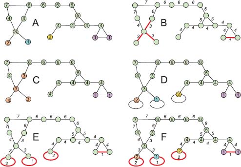
Figure 5.1. a) The initial graph is node-weighted. The ordinary nodes are green; each regional minimum is highlighted by a different color. b) The edge weights are obtained by dilating the node weights in A: η = δ_enν. The edges in red are the regional minima edges. Their extremities do not correspond to the regional minima of the node-weighted graph A. c) The node weights are obtained by eroding the edge weights in B: ν′ = ε_neη = ε_neδ_enν = φ_nν. All nodes retrieve their initial weight, except the isolated regional minima nodes. The new regional minima are not the same as in A. d) A loop edge has been added to each isolated regional minimum edge. e) The edge weights are obtained by dilating the node weights in D: η′ = δ_enν. The loop edges linking the isolated regional minima with themselves also get weights. The edges in red are the regional minima edges and now do correspond to the regional minima of the node-weighted graph A. f) the node weights are obtained by eroding the edge weights in E: ν” = ε_neη′ = ε_neδ_enν = φ_nν. All nodes retrieve their initial weight, including the isolated regional minima. The new regional minima are the same as the initial ones and are the extremities of the edge-based regional minima (in red). The resulting graph is a flowing graph. For a color version of the figures in this chapter, see www.iste.co.uk/meyer/topographical1.zip

The operator ε_neη assigns to each node the weight of its adjacent flowing edges. Hence, suppressing the non-flowing edges in the graph G(nil, η) does not modify the erosion ε_neη, i.e. the weight of the nodes.

LEMMA 5.5.– Suppressing all edges of the graph G(nil, η) whose weight is lowered by the opening γ_e produces a graph where each edge is a flowing edge with a weight invariant by γ_e. Both graphs have the same regional minima and catchment zones.

PROOF.– As shown above, the non-flowing edges are lowered by the opening γ_e, whereas the flowing edges are not. Hence, suppressing the edges lowered by γ_e leaves only the flowing edges. As a drop of water never follows a non-flowing edge, the flowing paths are not modified if such edges are cut. The regional minima are not modified either, as their inside edges are all flowing edges. Hence, the new graph ↓ G(nil, η) has the same catchment zones as the initial graph.

□

Hence:

PROPOSITION 5.4.– The graph ↓ G(nil, η) obtained by suppressing the non-flowing edges in an arbitrary graph G(nil, η) is a flowing graph. Its edge weights are invariant by γ_e : γ_eη = η.

Setting ν = δ_enν yields η = γ_eη = δ_enε_neη = δ_enν, establishing the perfect coupling between node and edge weights in the graph ↓ G(ε_neη, η), characterizing flowing graphs. The flowing edges, flowing paths, regional minima and catchment zones are identical in G(nil, η), ↓ G(nil, η) and ↓ G(ε_neη, nil).

Illustration

Figure 5.2 shows how to transform an edge-weighted graph G(nil, η) into a flowing graph. The initial graph in Figure 5.2(a) is edge-weighted with edge weights η. Its node weights ν are obtained by the erosion ε_ne : ν = ε_neη in Figure 5.2(b). Dilating these node weights produces new edge weights η′ = δ_enε_neη = γ_eη in Figure 5.2(c). The function η′ is the result of the opening γ_e applied to the function η. The weights of the edges which have been lowered are indicated in pink color. Such edges are not the lowest edge of one of their extremities. These edges have been suppressed in Figure 5.2(d), producing the flowing graph ↓ G(nil, η). This graph contains all edges of the initial graph which are the lowest edge of one of their extremities. Hence, the node weights still verify the relation ν = ε_neη in Figure 5.2(f). The graphs ↓ G(nil, η) in Figure 5.2(d) and ↓ G(ε_ne, nil) in Figure 5.2(e) have the same flowing edges, regional minima and catchment zones. The node weights and edge weights of the graph ↓ G(ε_neη, η) are represented in Figure 5.2(f). The inside edges of the regional minima are identical with those in the initial graph G(nil, η) in Figure 5.2(a). The extremities of these edges have been labeled, each regional minimum holding a different label.

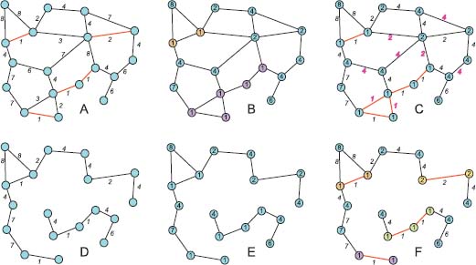
Figure 5.2. a) The initial graph is edge-weighted. The node weights are obtained by the erosion ε_ne: ν = ε_neη. b) The new edge weights are obtained by dilating the node weights in A: η′ = δ_enε_neη = γ_eη. Thus, η′ is obtained by the opening η applied to the edge weights of A. c) All edges of the initial graph A whose weight has been lowered by the opening γ_e, i.e. γ_eη < η are suppressed. The resulting graph is a flowing graph

5.4.7. Particular flowing graphs

5.4.7.1. The flowing graph ↻ G(ν, nil)

Linking each isolated regional minimum with itself creates the flowing graph ↻ G(ν, nil). In this new graph, the unchanged node weights verify ν = φ_nν. The graph ↻ G(nil, δ_enν) is then also a flowing graph with the same flowing edges. If we set η = δ_enν, the node- and edge-weighted graph ↻ G(ν, η) is also a flowing graph.

5.4.7.2. The flowing graph ↓ G(nil, η)

Suppressing each edge which is not the lowest edge for one of its extremities, i.e. edges for which η > γ_eη produces the flowing graph ↓ G(nil, η). In this new graph, the unchanged edge weights verify η = γ_eη. The graph ↓ G(ε_neη, nil) is then also a flowing graph with the same flowing edges. If we set ν = ε_neη, the node- and edge-weighted graph ↓ G(ν, η) is also a flowing graph.

5.4.7.3. The flowing graph G(ε_neη, nil)

As for any adjunction (δ_enε_ne), the erosion ε_neη is closed by the closing φ_n : φ_nε_neη = ε_neδ_enε_neη . Hence, G(ε_neη, nil) is a flowing graph with the same flowing edges as the graph G(nil, δ_enε_neη) = G(nil, γ_eη). If we set ν = ε_neη, the node- and edge-weighted graph ↓ G(ν, η) is also a flowing graph.

If η is not open by γ_e, the graphs G(nil, η) and G(nil, γ_eη) have distinct weights and distinct flowing paths. An edge which is not the lowest edge of one of its extremities is not a flowing edge in G(nil, η), but it is in G(nil, γ_eη).

5.4.7.4. The flowing graph G(nil, δ_enν)

As for any adjunction (δ_enε_ne), the dilation δ_enν is open by the opening γ_e : γ_eδ_enν = δ_enε_neδ_enν. Hence, G(nil, δ_enν) is a flowing graph with the same flowing edges as the graph G(ε_neδ_enν, nil) = G(φ_nν, nil). If we set η = δ_enν, the node- and edge-weighted graph ↻ G(ν, η) is also a flowing graph.

If ν is not closed by φ_n, the graphs G(ν, nil) and G(φ_nν, nil) have distinct weights and distinct flowing paths. An isolated regional minimum node in G(ν, nil) is not the origin of a flowing edge in G(ν, nil), but it is in G(φ_nν, nil).

5.5. Illustration as a hydrographic model

5.5.1. A hydrographic model of tanks and pipes

We now give a physical interpretation to the results of the last section. We represent a node- and edge-weighted graph G(ν, η) as a network of tanks linked by pipes.

We consider the nodes as vertical tanks of infinite height and depth. The weight ν_i represents the level of water in the tank i, which is equal to – ∞ if no water is present. Two neighboring tanks i and j are linked by a pipe at an altitude η_ij equal to the weight of the edge. Thus, an edge-weighted graph may be represented as a tank network, in which the interrelations between nodes and edges will be modeled as an hydrostatic equilibrium of water in the tank network.

For arbitrary weights of nodes and edges, the distribution of water does not follow the laws of hydrostatics. To represent a physically possible distribution of water, edge and node weights have to be coupled [MEY 13a, MEY 13b]: the level ν_i in the tank i cannot be higher than the level ν_j, unless η_ij ≥ ν_i. If two neighboring nodes and the pipe linking them verify this simple condition, the water distribution in our network is at equilibrium.

DEFINITION 5.4.– The distribution ν of water in the tanks of the graph G is a flooding of this graph, i.e. it is a stable distribution of fluid if it verifies the criterion hydrostat 1: for any couple of neighboring nodes (p, q): (ν_p > ν_q ⇒ η_pq ≥ ν_p)

Figure 5.3 presents several configurations compatible with the laws of hydrostatics and others which are not.

Figure 5.3. A tank and pipe network, in which the tanks (a, b…, f) verify the laws of hydrostatics, whereas the tanks (g, h) and (i, j) do not: – a and b form a regional minimum with τ_a = τ_b = λ; η_ab < λ; η_bc > λ; – b and c have unequal levels but are separated by a higher pipe; – d and e form a full lake, reaching the level of its lowest exhaust pipe η_cd; – e and f have the same level; however, they do not form a lake, as they are linked by a pipe which is higher

The following equivalences yield other useful criteria for recognizing flood distributions on tank networks:

On the contrary, (ν_p > ν_q ⇒ η_pq ≥ ν_p) ⇔ (η_pq < ν_p ⇒ ν_p ≥ ν_q).

If follows from the second implication: η_pq < ν_p ⇒ ν_p ≤ ν_p ⇒ η_pq < ν_p ≤ ν_q ⇒ ν_q ≤ ν_p. Putting everything together, we obtain η_pq < ν_p ⇒ ν_p = ν_q, showing that if the level ν_p in the tank p is higher than the pipe η_pq, then ν_p = ν_q, which is indeed the case for a hydrostatic equilibrium.

5.5.1.1. Critical fillings of a tank network

Consider a tank network representing a node- and edge-weighted graph G(ν, η). We suppose that its filling is at hydrostatic equilibrium, its node and edge weights verifying the criterion hydrostat 1. This equilibrium may be unstable:

• – It is “node unstable” if adding a drop of water in a tank produces an overflow into the lowest adjacent pipe, at level ε_neη.
• – It is “edge unstable” if lowering the edge level of a pipe (below the highest level of water δ_enν in the adjacent tanks) produces an overflow through this pipe.
• – It is “totally unstable”, if it is both node and edge unstable. In this case, we have a perfect coupling between the node and edge weights. As we will see below, the tank network is totally unstable if the corresponding graph G(ν, η) is a flowing graph.

5.5.2. Associating an “edge unstable” tank network with an arbitrary node-weighted graph G(ν, nil)

Given a node-weighted graph G(ν, nil), we associate with each node q a tank in which the water takes the altitude ν_q. If p and q are neighboring nodes in the graph, we set the pipe linking both tanks at the lowest possible level such that no water flows through the pipe. For two tanks p and q with water levels ν_p and ν_q, this pipe has to be set at a level η_pq = ν_p ∨ ν_q = (δ_enν)_pq. The distribution of water in the resulting tank network follows the laws of hydrostatics: as η_pq = ν_p ∨ ν_q, we have ν_p ≤ ν_q ∨ η_pq and ν_q ≤ ν_p ∨ η_pq, showing that the criterion hydrostat 2 is satisfied.

The resulting filling is “edge unstable”: if η_pq = ν_p ∨ ν_q and ν_p ≥ ν_q, lowering the level of η_pq would allow some water to enter into the pipe e_pq.

It is, however, not a “node unstable” filling. If m is an isolated regional minimum of the graph, each adjacent pipe will be placed at the level of a neighboring tank of m, i.e. at a higher level than ν_m. It is then possible to add a drop of water into the pipe m without provoking an overflow.

This is shown in Figure 5.4. Figure 5.4(1) represents the tanks corresponding to the graph G(ν, nil) (two neighboring nodes in the graph are represented as two neighboring tanks in the figure). Each tank is filled at a level equal to its node weight. In Figure 5.4(2), the neighboring tanks are linked by a pipe, placed at a level η_pq = ν_p ∨ ν_q for two neighboring tanks p and q. This tank network represents the graph G(ν, δ_enν).

Figure 5.4. The graph G(ν, δ_enν) is edge unstable but not necessarily node unstable: 1) Each tank represents a node of the graph G(ν, nil), filled to the level ν. 2) Pipes link the tanks corresponding to neighboring nodes in the graph G(ν, δ_enν); the pipe e_pq is placed at the level (δ_enν)_pq. The resulting network is edge unstable, as lowering the edge level of a pipe produces an overflow through this pipe. 3) The tank network representing G(ν, δ_enν) is not node unstable, as it is possible to add a drop of water into the tank c, representing an isolated regional minimum, without provoking an overflow through an adjacent pipe

Figure 5.4(3) shows what happens if we add a drop of water in any of the tanks. Adding a drop of water in the tank a provokes an overflow from a to b through the pipe e_ab which links them. The pipe f belongs to a non-isolated regional minimum containing two nodes f and g. Adding a drop of water in the tank f provokes an overflow from f to g through the pipe e_fg which links them. The node C is an isolated regional minimum, as all its neighboring nodes have higher weights. The graph is not “node unstable” as adding a drop of water in such an isolated regional minimum does not produce an overflow, since there is no pipe in the network at this level, but slightly increases the level of the water in the tank c. However, the resulting node- and edge-weighted graph is edge unstable, as lowering any edge would provoke an overflow through this edge from one of its extremities.

5.5.3. Associating a “node unstable” tank network with an arbitrary edge-weighted graph G(nil, η)

Consider now an edge-weighted graph G(nil, η). If p and q are neighboring nodes in the graph, then their associated tanks are linked by a pipe at level η_pq. We then fill the tanks as much as possible, again without creating any flow through the pipes. Obviously, if the level of water in a tank is higher than the level of one of its adjacent pipes, water will flow through this pipe. Therefore, the highest level ν_p of water in a tank p has to be equal to the level of the lowest adjacent pipe: . Adding a drop of water in the tank p would then provoke an overflow through this lowest adjacent pipe. The distribution of water in the resulting tank network then follows the laws of hydrostatics. Indeed, if p and q are two neighboring nodes 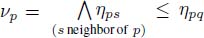and , then ν_p ≤ ν_q ∨ η_pq and ν_q ≤ ν_p ∨ η_pq, showing that the criterion hydrostat 2 is satisfied. The resulting tank network represents the graph G(ε_neη, η). It is “node unstable”.

However, it is not an “edge unstable” filling as shown by the counter example in Figure 5.5.

Figure 5.5(1) represents a tank network modeling an edge-weighted graph G(nil, η). Initially, the tanks are empty; the tanks corresponding to neighboring nodes are linked by a pipe set at an altitude equal to the weight of this edge. The nodes (f, g) and (b, c) form two regional minima. We verify that no isolated regional minima do exist in an edge-weighted graph. In Figure 5.5(2), each tank has been filled up to its lowest adjacent pipe. Figure 5.5(3) shows what happens if we add a drop of water in the tanks. Adding a drop of water in the tank c provokes a flow through the pipe linking c with the node b within the same regional minimum. Adding a drop of water in the tank e provokes a flow through the lowest adjacent edge towards the tank f. Similarly, adding a drop of water in the tank d would provoke a flow through the pipe linking d and c. The same happens for all tanks, as each of them has an adjacent pipe at the level of its filling, and adding a drop of water to the tank provokes an overflow through only this pipe. Therefore, the graph is “node unstable”.

Figure 5.5. The graph G(ε_neη, η) is node unstable but not necessarily edge unstable: 1) A network of tanks and pipes representing the graph G(nil, η); the pipe linking neighboring nodes p and q is placed at the level η_pq. 2) The tanks are filled up to their lowest adjacent pipe. Thus, adding a drop of water into a tank provokes an overflow through this lowest adjacent pipe. The tank network is node unstable. 3) However, the tank network representing G(ε_neη, η) is not edge unstable, as there are pipes which are not traversed by an overflow if we add a drop of water in one of the adjacent tanks. This is the case for the pipe e_de

In contrast, the pipe linking d and e is not the lowest pipe of its extremities and is never crossed by a flood if we add a drop of water in the network. Lowering the level of this edge also does not allow some water to pass through it. Hence, this graph is not “edge unstable”.

5.5.4. Chaining the operations

5.5.4.1. From node weights to edge weights and back on the graph G(ν, nil)

We first construct the tank and pipe network associated with a node-weighted graph G(ν, nil). The associated tank network is represented in Figure 5.6(1). We then produce the edge unstable filling G(ν, δ_enν) in Figure 5.6(2).

Forgetting the node weights, we obtain the edge-weighted graph G(nil, δ_enν) represented in Figure 5.6(4). The node unstable filling of this graph G(ε_neδ_enν, δ_enν) = G(φ_nν, δ_enν) is represented by the tank network in Figure 5.6(5). Adding a drop of water in the tank c in Figure 5.6(3) does not provoke an overflow into a neighboring pipe, whereas the same operation performed in Figure 5.6(5) produces an overflow through the pipe linking the tanks b and c.

In Figure 5.6(6), we compare the tank fillings of G(ν, nil) and of G(φ_nν, nil), showing that the isolated regional minimum node c has been filled up to the level of its lower neighboring node.

If ν is not closed by the closing φ_n, we have φ_nν > ν on all isolated regional minima. The succession of operations ν → δ_enν → ε_neδ_enν, transforming the node weights into edge weights and then back from the edge weights to the node weights is not equal to identity.

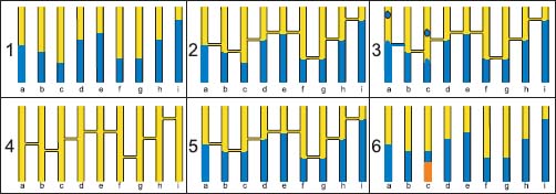
Figure 5.6. We represent a node-weighted graph G(ν, nil) by the tanks in image 1, connected by pipes at level δ_enν in image 2. The resulting graph G(ν, δ_enν) is not node unstable as shown in image 3: a drop of water is added into the tank c, representing an isolated regional minimum, without provoking an overflow. Image 4 represents the graph G(nil, δ_enν); each tank is filled up to the level ε_neδ_enν = φ_nν in image 5. Comparing the fillings of the tanks in images 1 and 5 shows that the level of the isolated regional minimum c has been filled up to its lowest adjacent node. Image 6 shows the initial level of water in pipe c in red and the final level in blue

5.5.4.2. From node weights to edge weights and back on the graph ↻ G(ν, nil)

We now transform the node-weighted graph G(ν, nil) into the graph ↻ G(ν, nil) by adding a loop edge linking each isolated regional minimum with itself.

The graph G(ν, nil) is represented in Figure 5.7(1) and ↻ G(ν, δ_enν) in Figure 5.7(2). A loop edge has been added to the isolated regional minimum of node c. Adding a drop of water in the corresponding tank allows water to enter into this pipe. The resulting tank network is also node unstable, as adding a drop of water in any of the tanks allows some water to enter into an adjacent pipe.

Forgetting the node weights, we obtain the edge-weighted graph ↻ G(nil, δ_enν) represented in Figure 5.7(4). The node unstable filling of this graph ↻ G(ε_neδ_enν, δ_enν) = ↻ G(φ_nν, δ_enν) is represented by the tank network in Figure 5.7(5). In Figure 5.7(6), we verify that the tank fillings of G(ν, nil) and ↻ G(φ_nν, nil) are identical. This is due to the fact that whatever the function ν in G(ν, nil), this function is closed by the closing φ_n in the graph ↻ G(ν, nil).

In the graph ↻ G(ν, nil), the succession of operations ν → δ_enν → ε_neδ_enν, transforming the node weights into edge weights and then back from the edge weights to the node weights is equal to identity, showing that the edge weights may be derived from the node weights and the node weights from the edge weights. If we set η = δ_enν, we have ν = ε_neη. The resulting graph is a flowing graph.

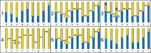
Figure 5.7. We represent a node-weighted graph G(ν, nil) by the tanks in image 1. The tanks are connected by pipes at level δ_enν in image 2; a pipe links the regional minimum tank c with itself, at the level ν_c. The resulting graph ↻ G(ν, δ_enν) is now node unstable as shown in image 3: a drop of water added into the tank c provokes an overflow through the pipe. Image 4 represents the graph ↻ G(nil, δ_enν); each tank is filled up to the level ε_neδ_enν = φ_nν in image 5. Comparing the fillings of the tanks in images 1 and 6 is now identical, as the graph ↻ G(ν, δ_enν) is a flowing graph.

5.5.4.3. From edge weights to node weights and back on the graph G(nil, η)

We first construct the tank and pipe network associated with an edge-weighted graph G(nil, η). The associated tank network is represented in Figure 5.8(1). We then produce the node unstable filling G(ε_neη, η) in Figure 5.8(2).

Forgetting the edge weights, we obtain the node-weighted graph G(ε_neη, nil) represented in Figure 5.8(4). The edge unstable filling of this graph G(ε_neη, δ_neε_neη) = G(ε_neη, γ_eη) is represented by the tank network in Figure 5.8(5). In Figure 5.8(6), we compare the levels of the pipes in G(nil, η) and G(nil, γeη), showing that the edge e_cd has been lowered. This edge is not the lowest edge of any of its extremities in G(nil, η).

If η is not open by the opening γ_e, we have γ_eη < η on all edges which are not flowing edges. The succession of operations η → ε_neη → δ_neε_neη, transforming the edge weights into node weights and then back from the node weights to the edge weights is not equal to identity.

Figure 5.8. We represent an edge-weighted graph G(nil, η) by the tank network in image 1. The tanks are filled at level ε_neη in image 2. The resulting graph (ε_neη, η) is now node unstable but not edge unstable, as there are pipes which are not traversed by an overflow if we add a drop of water in one of the adjacent tanks. This is the case for the pipe ed_e. Image 4 represents the graph G(ε_neη, nil). The tanks are linked by pipes at the level δ_enε_neη = γ_eν in image 5. Comparing the levels of the pipes in images 1 and 6 shows that the pipe e_de has been lowered, as the corresponding edge was not the lowest edge of one of its extremities

5.5.4.4. From node weights to edge weights and back on the graph ↓ G(nil, η)

We now transform the edge-weighted graph G(nil, η) into the graph ↓ G(nil, η) by cutting all edges which are not the lowest edge of one of their extremities; in our case, the edge e_de is cut. The graph G(nil, η) is represented in Figure 5.9(1) and ↓ G(nil, η) in Figure 5.9(2). The node unstable filling of the tanks produces Figure 5.9(3), representing the graph ↓ G(ε_neη, η).

Forgetting the edge weights, we obtain the node-weighted graph ↓ G(ε_neη, nil) represented in Figure 5.9(4). The edge unstable filling of this graph ↓ G(ε_neη, δ_enε_neη) =↓ G(ε_neη, γ_eη) is represented by the tank network in Figure 5.9(5). In Figure 5.9(6), we verify that the edge weights of ↓ G(nil, η) and ↓ G(nil, γ_eη) are identical. This is due to the fact that whatever the function η in G(nil, η), this function is open by the opening γ_e in the graph ↓ G(nil, η).

In the graph ↓ G(nil, η), the succession of operations η → ε_neη → δ_enε_neη, transforming the edge weights into node weights and then back from the node weights to the edge weights is equal to identity, showing that the node weights may be derived from the edge weights and the edge weights from the node weights. If we set ν = ε_neη, we have η = δ_enν. The resulting graph ↓ G(ν, η) is a flowing graph.

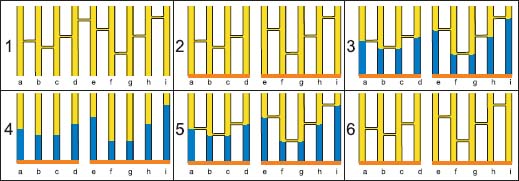
Figure 5.9. We represent an edge-weighted graph G(nil, η) by the tank network in image 1. The pipe e_de which is not the lowest pipe of one of its extremities is cut, producing the tank network associated with the graph ↓ G(nil, η) in image 2. In image 3, each tank is filled up to the level of its lowest adjacent edge, producing the graph ↓ G(ε_neη, η). Forgettting the pipes, we obtain the node-weighted graph ↓ G(ε_neη, nil) in image 4. The tanks are linked by pipes at the level δ_enε_neη = γ_eη in image 5 representing the graph ↓ G(ε_neη, δ_enε_neη). Forgetting the node weights in image 6, we obtain the graph ↓ G(nil, δ_enε_neη) whose pipes are at the same levels as the pipes in image 2 representing the graph ↓ G(nil, η)