8
Pruning a Flow Digraph

8.1. Summary of the chapter

8.1.1. Transforming a node- or edge-weighted graph into a node-weighted flowing digraph (reminder)

We have shown in the preceding chapters how any node- or edge-weighted graph may be transformed into a node-weighted digraph with the same flowing paths as the initial graph.

In a node-weighted graph G(ν, nil), each edge is a flowing edge and is transformed into an arc in the derived flow digraph , with the nodes keeping their weights.

An edge-weighted graph G(nil, η) is first transformed into a flowing graph ↓ G(nil, η) by cutting all edges, which are not the lowest edge of one of their extremities. This graph has the same flowing edges and paths as the node-weighted graph ↓ G(ε_neη, nil). We then replace the flowing edges with arcs with the same orientation and obtain a gravitational node-weighted digraph .

It appears that in both cases, whether we start from a node-weighted graph or an edge-weighted graph, we derive a node-weighted digraph whose directed paths are identical to the flowing paths of the initial graphs. In all cases we denote this graph by : equal to if the initial graph is G(ν, nil); equal to if the initial graph is G(nil, η)).

For the remainder of this chapter, we consider a node-weighted flow digraph and indifferently write , whether it has been derived from a node- or an edge-weighted graph. Its directed paths are identical to the flowing paths of the initial graphs.

8.1.2. Global pruning

In this chapter, we introduce a pruning operator, which increases the steepness of a node-weighted digraph, by cutting several arcs. The pruning is obtained by alternatively applying two operators on a node-weighted digraph:

• – The directed erosion assigns to each node p the minimal weight of its downstream neighbors: . It shifts the node weights upstream along directed paths. It does not cut arcs.
• – The scissor operator ↓² prunes digraphs, keeping all arcs (p → q) of origin p such that ν_q is minimal and suppresses all others. It does not affect the node weights. We showed earlier that this is authorized pruning. As such, it preserves the black holes of the unweighted digraph.

The unweighted digraph resulting from the pruning remains a gravitational digraph with the same black holes as the initial graph; its catchment zones, however, are not identical, as some directed paths have been cut. This property results from the fact that the coupling {p → q} ⇒ {ν_p ≥ ν_q} between arcs and node weights is preserved by the pruning: this property is verified for the initial node-weighted digraph and remains true every time we apply the operator ↓² .

We then establish that the pruning operator transforms a node-weighted digraph into an (n + 2)-steep digraph.

8.1.3. Local pruning

By applying ↓ⁿ, the first edges of all flowing paths which are not at least n – steep are cut. The operators ↓² and are local operators. Their arguments are the extremities of the arcs of the digraph and their weights. The pruning operator considers the n first nodes of the flowing paths with the same origin and cuts the first arc of the flowing paths which are not at least (n + 1) – steep. We call the union of the directed paths having p as the origin and as the union of the directed paths that have their origin in X.

Being a subgraph of , is also a gravitational graph, on which black holes and catchment zones may be detected.

8.2. The pruning operator

We now present a method for pruning a flow digraph, based on two neighborhood operators that preserve the ∞ – steep paths and cut the first edge of the others. One operator, , allows the weights move upstream along the flowing paths. The second, ↓², cuts arcs that are not the first edge of the less steep flowing paths. If applied to a k – steep digraph, the operator ↓² produces a (k + 1) – steep digraph.

As a result, several arcs will be cut and the node weights will be modified.

Note that the pruning uses the arcs of the digraph and its node weights. The topography of the pruned digraph, on the contrary, is then analyzed by considering only the arcs of the digraph, without considering the node weights. It appears that the black holes remain unchanged by the pruning, whereas the catchment zones become smaller and overlap less.

8.2.1. Two operators on flow digraphs

Pruning is achieved by alternatively applying the following operators that transform node-weighted digraphs into node-weighted digraphs. We consider a node-weighted digraph .

8.2.1.1. The scissor ↓²

The scissor operator ↓² prunes digraphs, keeping all arcs (p → q) of origin p such that ν_q is minimal and suppresses all others. We showed in lemma 6.6 that the operator ↓² is authorized pruning, i.e. all black holes are unchanged, without suppressing some of them or creating new ones.

Furthermore, if the digraph is a flow digraph before pruning ↓², it still is a flow digraph after pruning. Indeed, as the operator ↓² only suppresses arcs, the implication {p → q} ⇒ {ν_p ≥ ν_q} valid before pruning is still valid if some arcs have been cut.

8.2.1.2 The erosion

The directed erosion assigns to each node p the minimal weight of its downstream neighbors: . This operator is an erosion. If p has no lower neighboring node q such that p → q, we define .

LEMMA 8.1.– If is a flow digraph, i.e. verifies {p → q} ⇒ {ν_p ≥ ν_q}, then

PROOF.– If q is the lowest neighboring node of p such that (p → q), then . But {p → q} ⇒ {ν_p ≥ ν_q}, i.e. .

□

However, eroding a flow digraph with the operator does not necessarily produce a flow digraph as shown in the following example. Consider the node p in the flow digraph:

After erosion , node p has a weight equal to 1 and has an arc towards its left neighbor with the higher weight 3:

8.2.2. Pruning by concatenating both operators

8.2.2.1. Erosion followed by pruning

The operator does not preserve the property of a digraph to be flow digraph when it is used alone. However, if is applied after the operator ↓², then they form the operator ↓², which transforms a flow digraph into a flow digraph.

LEMMA 8.2.– The operator ↓² transforms a flow digraph into a flow digraph.

PROOF.– We first remark that after applying the operator ↓², all neighbors of node p verifying (p → q) have the same weight. Hence, the subsequent operator may assign to p the weight of any node t such that (p → t), without the need to consider all of them: . The relation being always true, we get . Hence, after ↓², the digraph is still a flow digraph, as

□

PROPOSITION 8.1.– The operator ↓² applied to a node-weighted flow digraph transforms it into a node-weighted flow digraph with the same black holes and reduced catchment zones.

PROOF.– We apply the operator ↓² to a node-weighted flow digraph. The first operator ↓² is authorized pruning. It preserves the black holes of the digraph. We recall that the black holes are detected by considering only the arcs and not the weights of the nodes. The subsequent operator only affects the node weights without touching the arcs. Thus, the black holes remain unchanged in the digraph ↓² .

Furthermore, as shown previously, the operator ↓² transforms a flowing digraph into a flowing digraph, and hence into a gravitational digraph. We know that in a gravitational digraph, each node is linked with a black hole and belongs to a catchment zone. As some arcs have been cut, some nodes stop belonging to the catchment zone of some black holes. However, they remain to the catchment zone of at least one black hole, as the graph produced by the pruning remains a gravitational graph.

□

REMARK 8.13.– The operator allows the node weights to migrate upstream along the directed paths of the digraph. Thus, the regional minima of the node weights become increasingly large. On the contrary, the black holes which do not rely on the node weights but only on the structure of the arcs remain unchanged.

8.2.2.2. The iterated pruning operator

Both operators, which can be alternatively used, are able to construct k – steep digraphs.

THEOREM 8.1.– If is a flow digraph, then is an (n + 2) – steep flow digraph. We call this operator .

PROOF.– We will proceed by induction on the steepness index k in the pruning ↓^k:

1. a) the operator cuts all arcs that do not link a node with its lowest neighbors. As a result, a 2-steep digraph is produced;
2. b) we suppose now that the operator produces a k + 1 steep digraph, i.e. each flowing path is at least (k + 1) – steep. We now prove that after an additional operator ↓² , the digraph will be (k + 2) – steep.

Consider three nodes p, q and s such that p → s and p → q . As each node, nodes s and q are, respectively, the origins of two ∞ – steep flowing paths σ and χ. We suppose, furthermore, that the path p ⊳ χ is ∞ – steep but p ⊳ σ is only (k + 1) – steep but not (k + 2) – steep.

The first edge of all flowing paths that are not at least (k + 1) – steep have been cut, but the first arcs p → s and p → q of p ⊳ σ and p ⊳ σ have been preserved, as these paths are at least (k + 1) – steep.

Since the path p ⊳ σ is not (k + 2) – steep, its (k + 2)th node, equal to θ_k+1(s), is larger than the (k + 2)th node of p ⊳ χ equal to θ_k+1(q).

We first apply the operator . After applying the operator on , the weights of the nodes along each ∞ – steep have moved upstream by k positions, since the operator has been applied k times. Thus, ν_q = θ_k+1(q), ν_s = θ_k+1(s) and ν_p = θ_k+1(p) = θ_k(q).

Since ν_s = θ_k+1(s) > θ_k+1(q) = ν_q, the subsequent operator ↓² cuts the arc p → s.

Thus, the operator produces, indeed, a (k + 2) – steep digraph, in which each node p takes the weight θ_k+1(p).

□

8.2.2.3. Comments

We remark that:

• – the digraph is ∞ – steep when an additional step of pruning does not change the result: ;
• – the pruning is obtained by a product of operators. If n = k + l, the pruning operator may be written as . The first operator produces the pruning ↓^l+2, and the last one completes the pruning and produces ↓^k+l+2. Thus, ;
• – each node outside a black hole is linked by at least one ∞ – steep path with a black hole. Such ∞ – steep paths remain unchanged by any pruning ↓^k regardless of the value of k.

8.2.2.4. Illustration

Figure 8.1(a) represents a flow digraph. The successive drawings of Figure 8.1 represent the evolution of the digraph during the successive operations, alternatively pruning ⇂² and eroding until stability. At each iteration, up to convergence, the catchment zones are reduced. At convergence, the catchment zones no longer overlap. Residual and tiny overlapping may nevertheless remain in some cases, as will be discussed later on in this book.

8.2.3. Properties of pruning

8.2.3.1. Flat zones in a k-steep digraph

Let us now analyze under which conditions double arcs may subsist in a k – steep digraph. Consider in Figure 8.3 a portion of a k – steep digraph. A double arc exists between nodes p and q. The arc (p → q) is the first arc of a flowing path π of origin p, and the arc (q → p) the first arc of a flowing path σ of origin q.

If the digraph π is k – steep, we have:

• – ∀l < k : θ_l+1(p) = θ_l (q) for the path π.
• – ∀l < k : θ_l+1(q) = θ_l (p) for the path σ.

Figure 8.1. Pruning of the digraph derived from a node-weighted graph. The evolution of a digraph under repeated use of the operator ⇂²: a) initial flow digraph . b) ⇂² in which the first arc has been cut. c) ⇂² : the node weights move in the opposite directions of the arrows. d) ⇂² ⇂² : a simple arc and two bidirectional arcs have been cut. e) . f) : each node now belongs to one and only one catchment zone. As a result, we get a 4 – steep digraph, which is in our case also a ∞ – steep digraph as each node outside the regional minima is the origin of a unique oriented path. For a color version of the Figures in this chapter, see www.iste.co.uk/meyer/topographical1.zip

Putting everything together, in the case where k is odd we have:

• θ_k(p) = θ_k–1(q) = θ_k–2(p) = θ_k–3(q) = …θ₁(p)
• θ_k(q) = θ_k–1(p) = θ_k–2(q) = θ_k–3(p) = …θ₁(q)

And in the case where k is even:

• θ_k(p) = θ_k–1(q) = θ_k–2(p) = θ_k–3(q) = …θ₁(q)
• θ_k(q) = θ_k–1(p) = θ_k–2(q) = θ_k–3(p) = …θ₁(p)

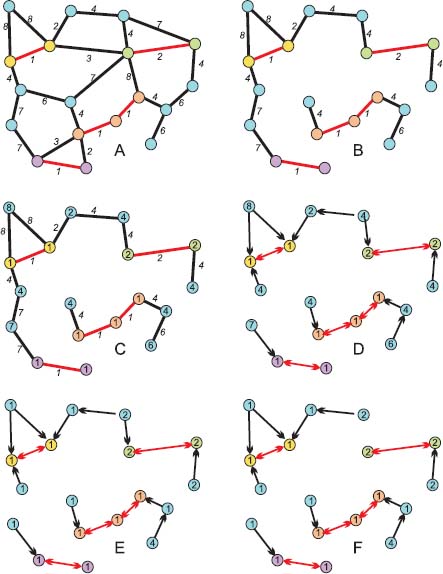
Figure 8.2. Starting from an edge-weighted graph, creation of a digraph and pruning: a) initial edge-weighted graph G; b) the corresponding flowing graph, in which the edges which are not the lowest edge of one of their extremities have been suppressed; c) the node weights have been obtained by applying the erosion ε_ne to the edge weights; d) the 2-steep digraph ⇂² has been obtained by creating an arc between each node and its lowest neighbors; e) ⇂² : the node weights move in the opposite directions of the arrows; f) ⇂² ⇂² : new edges have been cut. Each node belongs to one and only one catchment zone. As a result, we get a 3 – steep digraph, which is here also ∞ – steep, as only ∞ – steep flowing paths subsist

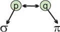
Figure 8.3. For a large enough k, there are no longer double arcs in the graph ⇂^k

Since a double arc exists between p and q, we have θ₁(p) = θ₁(q), showing that all weights ∀l ≤ k : θ_l(p) and θ_l(q) are equal. This shows that p and q belong to the interior of a plateau with a depth k.

This may happen in two situations:

• – both nodes belong to flat zones, but the distance of the nodes p and q is higher than k from the nearest node with a lower weight than p and q. Only a more severe pruning than k will suppress the bidirectional arc between p and q;
• – both nodes belong to the same black hole. In such a case, the path linking both nodes remains unchanged by pruning. This is the only possibility after an infinite pruning ⇂^∞.

8.2.3.2. Button holes

If there are no remaining double arcs in an ∞ – steep digraph, it does not mean that the overlapping zones have vanished or that they are only 1 node wide. Figure 8.4 shows a case where the node with weight 4 is the origin of two distinct flowing paths, reaching two black holes with a weight 1. The upstream of this node is called button hole; here, it contains six nodes belonging all to the catchment zones of the blue black hole.

Figure 8.4. A button hole: it is impossible, without some arbitrary choice, to attribute the green nodes to one of the regional minima with weight 1

8.2.4. A variant of pruning

Before comparing the steepness of the flowing paths with a given origin, these paths are prolonged into infinite path. The flowing path starting from a node p and ending at a node m of a black hole is prolonged by appending an infinite number of values. These values may be the weight of the black hole or simply the value o, minimal value of the ordered set T, in which the nodes take their value.

The pruning presented so far amounts at infinitely duplicating the weight of the black holes at the end of the directed paths. This is due to the definition of the operator 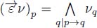. If a node p belongs to a non-isolated black hole, it has a neighbor s with the same weight verifying p → s. The weight of p remains thus unchanged. If p has no lower neighboring node q such that p → q, then 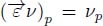. Again, the weight of p remains unchanged. Thus, each new application of allows these weights of the black holes to be propagated into the flowing paths.

If we wish to append an infinite series of o at the end of the flowing paths, we perform the first step of pruning: 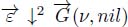, which allows the weights of the black hole to move upstream by one position. We then assign to all nodes belonging to a black hole of the weight o before continuing the pruning. Thus, each new application of allows these weights of the black holes to be propagated into the flowing paths.

If we denote by ô the operator assigning to the black holes the weight o, the modified pruning operator is then: .

8.2.5. Local pruning

8.2.5.1. The “comet”, union of flowing paths of lengths n that have their origin in X

The operators ↓² and both take as arguments the arcs and the weights of the nodes connected by an arc p → q. By applying ↓ⁿ, the first edges of all flowing paths, which are not at least n – steep, are cut.

In particular, whether the arcs of origin p are cut or not only depends on the n first nodes of the directed paths of origin p.

We call the union of these directed paths that have their origin in the set X and are reduced to their first n nodes. Being a subgraph of , is also a flow digraph.

We denote by the union of all directed paths that have their origin in X and their extremity in a black hole.

As a conclusion, the operator ↓ⁿ has the same effect on the flowing paths that have their origin in a set X, whether it is applied to the digraph or to . In particular, it cuts the first arcs of flowing paths that have their origin in X which are not at least n – steep.

8.2.5.2. Illustration

Figure 8.5(a) shows an edge-weighted graph G(nil, η) in which a node p has been highlighted with a red rim. We would like to find the steepest paths leading from this node to black holes. Figure 8.5(b) shows the associated flow digraph whose directed paths represent the flowing paths of G(nil, η). The directed paths of origin p constitute the subgraph , represented by Figure 8.5(c). The subdigraph is highlighted in Figure 8.5(b) with red rims.

As no arc is connected with other nodes compared to its lowest neighbors, is 2 – steep. The operator allows the weights to move upstream in , as shown in Figure 8.5(d). Finally, the operator ↓² cuts an arc leading from p to the violet black hole in Figure 8.5(e). After this pruning, the node p is only connected with the yellow black hole. Its downstream contains only one directed path leading to this minimum. The corresponding flowing path is highlighted in the original graph in Figure 8.5(f).

8.2.5.3. Factorization of global pruning into global and local pruning

The pruning may be decomposed into the product of two operators . The first pruning may be applied to the complete digraph which reduces the number of flowing paths of origin X. A second pruning (↓²)^k is then applied to , where X is the set of nodes whose downstream has to be pruned.

8.3. Evolution of the catchment zones with pruning

The effect of pruning clearly appears if we consider the downstream and the catchment basin of a particular node. The downstream of a node is the union of all flowing paths having this node as the origin. With higher intensities of pruning, the number of such paths is reduced.

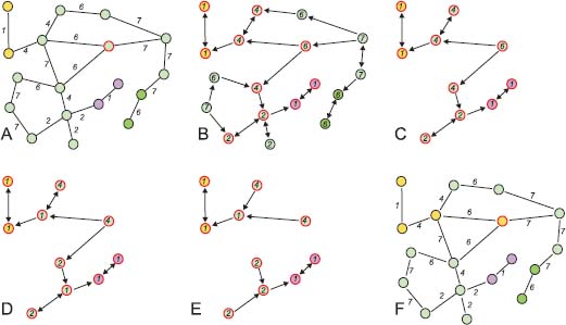
Figure 8.5. a) An edge-weighted graph G(nil, η), with the node p highlighted by a red rim; b) The corresponding digraph in which the directed paths of origin p have been highlighted by a red rim. c) They constitute the sub-digraph which is 2-steep. d) The erosion of is followed in E by the pruning ↓². The node p is now linked by an oriented path with only one black hole. e) The node p and the steepest flowing path linking p with a black hole in the graph G(nil, η) are highlighted in yellow on the nodes

The downstream of a node p ends within a black hole and entirely contains this black hole. Hence, the upstream of the downstream of p contains all catchment zones containing p. With increasing pruning intensities, the catchment zones become smaller and converge towards the minimal catchment zones associated with infinite pruning. This effect is well illustrated in Figure 8.6.

8.3.1. Analyzing a digital elevation model

8.3.1.1. The catchment zone of a marked region

Figure 8.6 shows a digital elevation model on which a set X is marked with a black dot. The flow digraph associated with the gray tone image has been constructed and submitted to various degrees of pruning. We compare, for increasing degrees of pruning, the result of a downstream propagation, on the one hand, and of the subsequent upstream propagation, on the other hand, of the label of the marked node

For each degree of pruning, we construct the downstream of the black marked dot, producing a river appearing in pink, ending at a regional minimum. A subsequent upstream propagation of the label reconstructs the catchment zone containing the black dot. The contour of the catchment zone appears with a red contour.

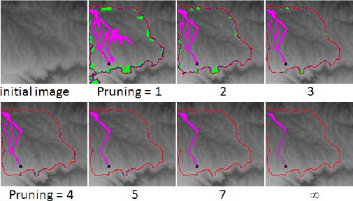
Figure 8.6. The flowing paths (in violet) and the catchment zone of the dark dot are compared for increasing degrees of pruning (1, 2, 3, 4, 5, 7, ∞)

Let us observe the evolution of both the rivers and the catchment zone for the degrees of pruning: k = 1, 2, 3, 4, 5, 7, ∞.

For small values of k, the river divides into several branches and is relatively large. As the pruning becomes more severe, the river narrows down, with less branches, until only one thin branch remains.

In parallel, the catchment zone becomes increasingly smaller with increasing degrees of pruning. The portion of the catchment zone overlapping with a neighboring one is indicated in green. We have explained in the chapter “The Topography of Digraphs” how such overlapping zones may be detected. We see that green zones become increasingly smaller when the pruning becomes more intense.

In practice, for such types of images, it seems that a pruning of intensity 7 would be sufficient for obtaining results similar to the best results associated with an infinite pruning.

Later, we present a direct method for delineating the overlapping zones between catchment zones and a local method for correcting the most prominent errors.

8.3.1.2. The dead leaves model of all catchment zones

In the previous sub-section, we have considered a single catchment zone. Here, we consider the catchment zones of all regional minima (black holes in the associated flow digraph), which have been assigned arbitrary labels, with an arbitrary priority order between the labels. Minima and priority order have in this application no particular meaning. We have submitted the flow digraph associated with the image to various degrees of pruning. For each pruned sub-digraph, we have propagated the labels upstream obtaining a dead leaves partition of the domain. The catchment zone with a higher priority covers the catchment zones with a lower priority. Each tile of the partition contains a regional minimum.

Figure 8.7 shows a partition into catchment zones of a topographic surface. The lower row shows the evolution of the frontier for increasing intensities of pruning. With higher degrees of pruning, the catchment zones overlap less. For k ≥ 5, the partitions are very close to the most precise we obtained for k = ∞.

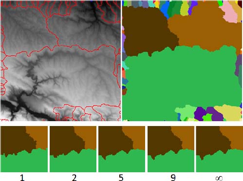
Figure 8.7. Catchment zones obtained for increasing pruning intensities

8.3.1.3. The Influence of pruning intensity on catchment zones during segmentation of a gradient image

Figure 8.8 shows a typical sequence of morphological segmentation. The image to be segmented is shown in Figure 8.8(a) and its gradient in Figure 8.8(b). A flow digraph is associated with the gradient image, and the regional minima are detected and labeled in Figure 8.8(c). Figure 8.8(d) shows a watershed partition of the gray tone image, each basin taking the label of its minimum. The watershed partition associated with the regional minima is obtained with the classical hierarchical queue-driven flooding algorithm [MEY 91] (this is the special case of the core-expanding algorithm presented in Chapter 9), which produces minimal overlapping between catchment zones. Figure 8.8(e) represents a mosaic image in which each tile of the watershed partition has been replaced by the mean gray tone of the initial image.

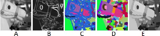
Figure 8.8. Typical sequence of segmentation. The watershed partition is obtained by the core-expanding algorithm driven by a hierarchical queue

We now replace the hierarchical queue watershed algorithm with a dead leaves tessellation of catchment zones obtained after pruning the digraph associated with the gradient image. We also analyze the evolution of overlapping when pruning becomes more severe.

We have chosen an arbitrary priority order between the labels and propagated these labels upstream with the operator ↗_∞. The resulting dead leaves partition is represented in the left column of Figure 8.9. We have then inverted the previous priority order between labels and again applied the operator ↗_∞, producing a new dead leaves partition represented in the central column of Figure 8.9. The dead leaves placed on the top in the left column are below all others in the right column. The discrepancies between the two partitions are highlighted in the right column. They become smaller with increasing degrees of pruning. It appears that for one and three pruning steps, the overlapping zones are significant. However, after five steps of pruning, the discrepancies are not significantly more important than the discrepancies obtained on an ∞ – steep digraph.

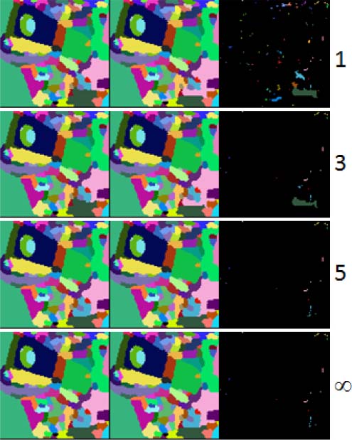
Figure 8.9. Comparison of the watershed partitions obtained by the upstream propagation of labels on a k – steep digraph for k = 1, 3, 5, ∞. For each degree of pruning, two partitions are produced: one on the left with a particular order relation between the labels and the other in the center with an inverted order relation. The rightmost figure presents the discrepancies between the two partitions, i.e. the zones where catchment zones overlap. The overlapping zones decrease with higher degrees of pruning and become practically stable after five steps of pruning

However, the overlapping zones do not completely vanish with infinite pruning. A node belongs to the catchment zones of two regional minima after infinite pruning if the flowing paths leading to these minima have identical weights. This is more likely to happen for small regions, as then the flowing paths are short.