12
Intermezzo: Encoding the Digraph Associated with an Image

12.1. Summary of the theoretical developments seen so far

In the previous chapters, we studied the topography or node- or edge-weighted graphs, by considering the possible trajectories of a drop of water from node to node on these graphs. A drop of water glides from a node p to a node q, if the edge e_pq is a flowing edge of p.

In a node-weighted graph G(ν, nil), each edge is a flowing edge of one of its extremities. In an edge-weighted graph G(nil, η), some edges are never crossed by a drop of water as they are not the flowing edge of one of their extremities. They may be suppressed without modifying the trajectories of a drop of water. The resulting graph ↓ G(nil, η) is a flowing graph. Such a graph has the same flowing edges as the corresponding node-weighted graph ↓ G(ε_neη, nil).

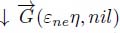These node-weighted graphs G(ν, nil) and ↓G(ε_neη, nil) are then transformed into node-weighted flow digraphs and , by replacing each flowing edge with an arrow, in the direction of the flow. We called these digraphs flow digraphs.

These node-weighted digraphs are then transformed into k – steep or ∞ – steep digraphs. These digraphs are gravitational digraphs in which the black holes and their catchment zones may be detected, considering only the arrows of the digraph, without taking into account the node weights. In order to label the various structures of the digraphs, labels are assigned to the nodes. These labels may then be propagated downstream in the direction of the arcs or upstream in the opposite direction.

12.2. Summary of the chapter

In order to implement these operators, we have to choose an appropriate encoding of the digraphs. There are many ways to represent graphs and digraphs described in the literature on graphs.

Images represented on a grid may, however, be considered as particular graphs, in which the pixels are the nodes, edges linking adjacent nodes. Figure 12.2 presents an image and the associated graph structure. While the graphs have an essentially flexible structure, it is not the case of images, which are defined on a fixed grid, with a crystallographic regularity. Each point in a grid has the same neighborhood structure, with the same number of neighbors at the same relative positions. The neighbors may thus be numbered. The n-th neighbor p of a node q may be encoded by setting to 1 the n-th bit of node q, indicating the presence of an arc between p and q.

In addition, each node may hold a label and a weight. All algorithms presented so far may then be applied to this particular representation of node-weighted digraphs.

In this chapter, we show how to encode the node-weighted digraphs representing images, taking advantage of their regular structure. We then revisit and illustrate for images the various operators defined earlier for extracting the regional minima, catchment zones and their overlapping.

12.3. Representing a node-weighted digraph as two images

12.3.1. The encoding of the digraph associated with an image

The grids on which images are represented have a regular structure, where each node has the same number of neighbors, in identical positions. The neighbors are numbered according to their direction to represent the neighborhood relations of each pixel with a binary number, where each bit encodes for one direction. The n-th bit is set to 1 if and only if an arrow exists between the central points towards its n-th neighbor; such arrows with node i as the origin are called out-arrows of i. Figure 12.1 shows the numbering of the directions for a hexagonal raster and the corresponding bit planes (on the right). The bottom image gives an example of encoding a particular neighborhood configuration. We consider arrows in the directions 1, 2 and 6, which produce the code 2⁰ +2¹ +2⁵ = 1+2+32 = 35. The same principle may be applied for any regular grid in any number of dimensions.

Figure 12.2 shows on its right side the arrows of the digraph associated with the gray tone image on its left side: an arrow is created between each node and its lower or equal neighbors; the regional minima having no outgoing arrows. In the case where two nodes are linked by a double arrow, an arrow will be created and the corresponding bit set at the node p in the direction of q and another arrow at the node q in the direction of p.

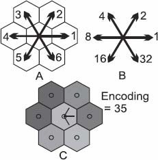
Figure 12.1. Encoding of the digraph: a) The six directions of the hexagonal grid. b) The direction i is encoded as 2^i-1. c) Encoding of the central node of the digraph, with an arrow towards all neighboring nodes with inferior or equal weights. The code is 2⁰ + 2¹ + 2⁵ = 1 + 2 + 32 = 35. For a color version of the figures in this chapter, see www.iste.co.uk/meyer/topographical1.zip

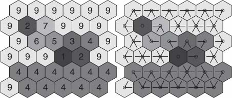
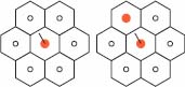
Figure 12.2. A gray tone image and the encoding of its flow digraph

We thus need three images for representing the digraph that represent an image. The first for the function ν. The second encodes the graph structure itself, i.e. the directions of the arcs that have a given node as the origin. In addition, we need a third image, encoding the labels of the nodes.

12.3.2. Operators acting on node-weighted digraphs

12.3.2.1. Erosion

Directed erosion considers for each node p the weight of the extremities of all arcs that have p as the origin; it assigns to p the smallest weight of these extremities. Figure 12.3 illustrates the erosion for three configurations. The first image in each row shows the gray tone distribution, the second image shows the out-arrows of the central pixel and the rightmost image shows the gray tone assigned to the central pixel by the erosion . Figure 12.3(c) is a case where no arrow is present at a pixel. In this case, the gray tone of the central pixel is preserved.

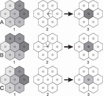
Figure 12.3. Illustration of the erosion for three different configurations A, B and C. The operator takes as input the gray tone image 1 and the image 2, encoding the arcs of the digraph. As a result, it assigns to each node the gray tone of its lowest exhaust node. This value is written in the gray tone image 3, and the image encoding the arcs is not modified

12.3.2.2. The scissor operator ⇂²

The scissor operator ⇂² considers all arcs that have a given node p as the origin. It keeps only those arcs pointing to the lowest neighbors of p. In other words: (p → q) is kept iff 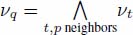. All other arcs with p as the origin are suppressed. Figure 12.4 illustrates the pruning operator for three different configurations. For each row, the leftmost image presents the gray tone distribution on a node and its neighborhood. The central image shows the distribution of arrows on the central pixel before the pruning. The leftmost image presents the distribution of arrows on the central pixel after the pruning. It is interesting to compare the rows A and B, which have the same gray tone distribution, but not the same distribution of arrows. In Figure 12.4(a), the pruning leaves an arrow towards the darkest node in the neighborhood, as an arrow existed in this direction before pruning. In Figure 12.4(b), on the contrary, the pruning leaves arrows towards the two nodes on the top which are the darkest nodes pointed to by an arrow. The very darkest node in the neighborhood had no arrow pointing to it before the pruning, and thus its value is discarded by pruning.

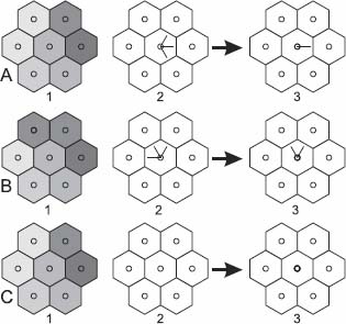
Figure 12.4. Illustration of the pruning ⇂² for three different configurations A, B and C. The operator takes as input the gray tone image 1 and the image 2, encoding the arcs of the digraph. This pruning considers all arrows with the same origin and suppresses all those whose exhaust node has not a minimal weight

Figure 12.6 and 12.7 present the same evolution for a gray tone image. In Figure 12.6, we represent the gray tone distribution of the image during the successive steps of pruning. Figure 12.7 presents the arcs that have their origin in each node as the pruning proceeds. More and more arcs are suppressed, reducing the catchment zones.

12.3.2.3. Pruning and eroding

Both operators and ⇂² may be chained as shown by Figure 12.5. Figure 12.5 presents on the left two configuration of a flow digraph, in which the node weights are represented by gray tones. From A to B, the pruning operator ⇂² has been applied and, from B to C, the result of the erosion on the central node.

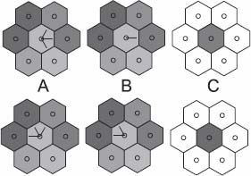
Figure 12.5. From A to B: pruning ⇂²; from B to C: erosion

The operator ⇂^k+2= (⇂² ) ⇂² prunes the digraph producing an (k + 2) – steep digraph. It converges for increasing values of k towards ∞– steep digraph. The gray tones of the regional minima move upstream along the ∞ – steep flowing paths. If a node p belongs to two catchment zones, it will take the gray tone of the smallest regional minimum. We obtain at convergence a partition of catchment basins, where each basin has the gray tone of its regional minimum.

Figure 12.6 presents a gray tone image, with its regional minima indicated by colored dots. The successive images show the evolution of the gray tone distribution and of the arrows during the successive steps of pruning. For a better visualization of the arrows, Figure 12.7 presents the same image submitted to successive steps of pruning without superimposing the gray tones on the arrows.

12.4. Defining labels

We need a third image, representing labels. Typically, the labels will serve to encode the various substructures extracted from the graph. All nodes belonging to the same substructure, for instance, a regional minimum, or a catchment zone, or a flowing path may then share the same label. Used for numbering and identifying structures, the labels are generally integers. Thus, the label function is defined on the nodes for a value of and belongs to . We therefore obtain a graph 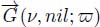represented by three images, as illustrated by Figure 12.8: a gray tone image representing the topographic surface, an image holding the arrows and the last image representing labels, for instance, of the regional minima or of the catchment basins in construction. A priority relation is defined between the labels. Thus, if a node belongs to different structures holding distinct labels, it is assigned the most prioritary label.

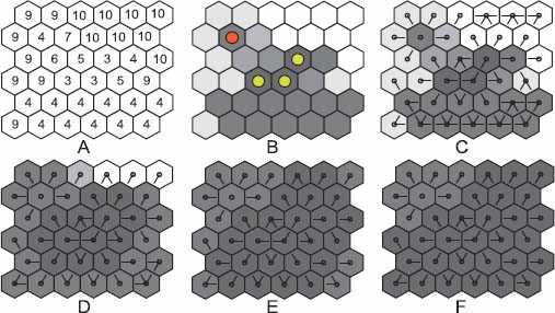
Figure 12.6. a) Initial gray tone image, with the corresponding gray tones in b) and both its regional minima with colored dots. c) Arrows link each node with its lowest neighbors. This corresponds to the first pruning ⇂² of the flow digraph. d) to f) Successive applications of the operator ⇂² , pruning the arrows and letting the gray tones move upstream along the ∞ — steep flowing paths. If the regional minima have distinct gray tones, we obtain a watershed partition

12.4.1. Operators on unweighted unlabeled digraphs

A simple operator operating on the digraph simply consists of inverting the arcs.

The inversion of arcs is an operator ξ which transforms each arc (q → p) into an arc (p → q). This operator ξ is able to construct dual operators. If ζ is an operator, its dual with respect to arrows is ξζξ . The downstream propagation, for instance, is dual of the upstream propagation. As another example, the dual of the black holes represent the regional maxima of the initial graphs.

Figure 12.7. a) Initial gray tone image, with the corresponding gray tones in b) and both its regional minima with colored dots. c) Arrows link each node with its lowest neighbors. This corresponds to the first pruning ⇂² of the flow digraph. d) to f) Successive applications of the operator , pruning the arrows and leaving the arrows of the black holes unchanged

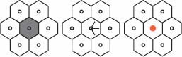
Figure 12.8. In the case of images, we have three images, the first expressing the gray tones of the pixels, the second encoding the arcs that have their origin in the central point and the last encoding labels

12.4.2. Operators on labeled unweighted digraphs

12.4.2.1. Label propagation

The labels may be propagated upstream or downstream as explained in the chapter on digraphs. The upstream operator is illustrated in Figure 12.10 in the case of images. We write for the upstream operator applied k times, and or if we apply it up to stability (more precisely up to the iteration n such that 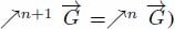. The downstream operator is illustrated in Figure 12.10 in the case of images. We write for the downstream operator applied k times, and or if we apply it up to stability (more precisely up to the iteration n such that .

Figure 12.9. From left to right: inversion of the arcs

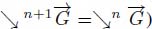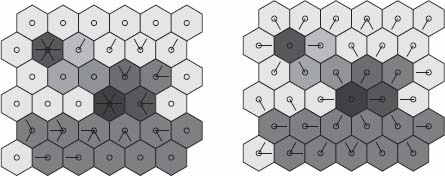
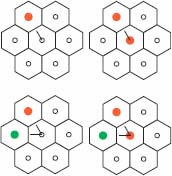
Figure 12.10. The upstream operator

Figure 12.11. The downstream operator

12.4.2.2. Illustration: upstream of downstream

The downstream and upstream operators are used here for extracting marked catchment zones. Figure 12.12(a) presents an unweighted and labeled digraph , in which a node has been attributed a positive label (in red). In Figure 12.12(b), the label has been propagated downstream: in blue, the downstream of the red node and, in green, the black hole where the flowing path ends. In Figure 12.12(c), a subsequent upstream propagation adds the nodes in gray color, reconstructing the catchment zone of the node marked red in Figure 12.12(a).

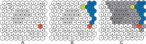
Figure 12.12. a): An unweighted and labeled digraph , in which a node has been attributed a label (in red); b): Downstream propagation of the labeled nodes: in blue, the downstream of the red node and, in green, the black hole at the end of the flowing path; c): Upstream propagation of the labels: the nodes which have been added are in gray color

12.4.2.3. Black hole detection on labeled unweighted digraphs

The black hole detection takes an unlabeled digraph as input, and detects and labels its regional minima. We presented the algorithm in the chapter on digraphs. We first detect the nodes which do not belong to a regional minimum. They are the upstream of the nodes p such that (p → q) and (q ↛ p). In Figure 12.13, we have represented on the left the set X of nodes p verifying (p → q) and (q ↛ p); these nodes have a white color. The other nodes have a gray color; among them are the regional minima nodes. On the right, we have represented the upstream of X in white. The complement of the upstream contains the black holes, appearing in red and green.

12.4.2.3.1. Detection of the overlapping zones on labeled unweighted digraphs

We consider a labeled flow digraph in which the labels form a partial partition, the result of the upstream label propagation of the labels of some marked nodes. If two nodes p, q verifying (p → q) hold distinct labels, the node p belongs to two distinct catchment zones. The label of q could not be propagated to the node p, as the label of q has a lower priority than the label of p. Such nodes are called “overlapping seeds”, forming a set S defined by:

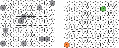
Figure 12.13. Left: The nodes defined by X = {p \ p, q ϵ N : (p → q) and (q ↛ p)} appear in white and their upstream are the complement of the black holes. Right: The labeled black holes are the complement of X and its upstream

The overlapping core is constituted by the upstream of the overlapping seeds.

Figure 12.14 illustrates the detection of the overlapping zones. Figure 12.14(a) shows a graph in which two regional minima (highlighted by a green and a yellow dot) are present. The minimum with the green dot is assigned a darker label and the minimum with the yellow dot is assigned a brighter label. These labels have been propagated upstream, the lighter label having a higher priority than the darker label. Hence, all nodes of the overlapping zone are labeled in light gray. In Figure 12.14(b), the overlapping seeds have been detected, which appear as red dots and their upstream as white dots. Together, the white and red dots form the domain where both catchment zones overlap.

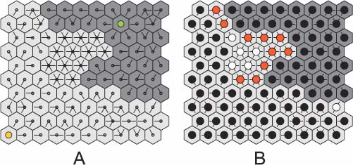
Figure 12.14. a) A graph , where two regional minima have been labeled and propagated upstream. The light gray labels have higher priority than the dark gray labels. Hence, the overlapping area of both labels is occupied by the light gray label. b) The overlapping seeds have been detected, which appears as red dots and their upstream as white dots. Together, the white and red dots form the overlapping core

12.4.3. Operators on weighted and labeled digraphs

12.4.3.1. Combining pruning and propagation of labels

Consider a flow digraph in which the black holes have been labeled. The pruning operator applies repeatedly the operator on the digraph . We may interleave the upstream propagation of the labels inside the pruning sequence: after each application of the operator ⇂², we apply the operator . Thus, the complete sequence is . The process stops when all nodes have been labeled, producing a dead leaves watershed partition. As the propagation of the labels occurred following ∞ — steep paths, the resulting catchment zones have minimal overlapping.

Figure 12.15 illustrates the process. Figure 12.15(a) and (b) presents a gray tone image, containing two regional minima. In Figure 12.15(b), these minima have been detected and labeled. In Figure 12.15(c), an arrow has been created between each node and its lowest neighbors, corresponding to the first pruning of the associated flow digraph . Figures 12.15(d) and (e) show the evolution of the labels during the subsequent sequence of operators . Figure 12.15(f) presents the final partition superimposed with the initial node weights.

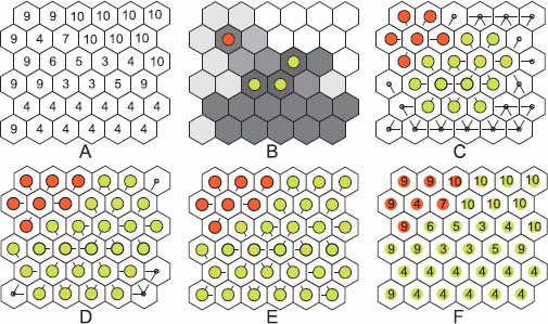
Figure 12.15. a) Initial gray tone image, with the corresponding gray tones in b) and both its regional minima with colored dots. c) Arrows link each node with its lowest neighbors. This corresponds to the first pruning ⇂² of the flow digraph. The labels have been propagated one step upstream. d) and e) Successive applications of the operator , pruning the arrows and propagating the labels. f) Final partition superimposed with the initial node weights

12.4.3.2. Detection of pass points on weighted and labeled digraphs

Consider a dead leaves watershed partition in which each region has a distinct label. We aim to detect the pass points between the various regions. A pass point has the same meaning as on a real topographic surface. It corresponds to an edge between neighboring nodes through which flooding covering one region may invade the second region. The level of the pass point is the minimal level for which an overflow may occur from a labeled region into a neighboring region.

Consider two neighboring regions, one with label and the other with label . The pass points between these regions are the couples of neighboring nodes (p, q), such that 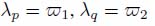for which the weight v_p V v_q is minimum.

The following method detects the pass points between the region with label and that with label .

For each node p with a label that has a node with label in its neighborhood; we create an arc (p → q), if q has the smallest weight among all neighboring nodes of p holding the label and assign to the node p the weight .

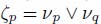The couple (s, t) is a pass point between the region with label and that with label , if s is the node with the smallest weight ζs and an arc has been created between s and t.

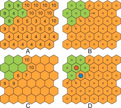
Figure 12.16. a) A watershed partition with two catchment basins. b) An arrow is created for each orange node with a green neighbor towards the green neighbor with the smallest weight. c) For each of these arrows (p → q), we assign to p the weight ν_p V ν_q. d) The arrows with an orange origin and with the lowest weight belong to the pass points between the orange catchment zone and its neighboring catchment zones, here the green one

Figure 12.16 presents a watershed partition with two catchment zones: a green and an orange one. We aim to detect the pass point between the two zones. In Figure 12.16(b), an arrow is created between each orange node and its lowest green neighbor (which may have a higher altitude than the origin). In Figure 12.16(c), we assign to each origin of an arrow the maximal weight between the origin and the extremity. The smallest weight is 6. The node with weight 6 appears in blue in Figure 12.16(d). It points towards a red node. Together, these nodes form a pass point between the orange and the green region.

If we wish to detect the pass point between a region and several of its neighboring regions, the previous method is trivially extended. We consider the inside region as one label and assign a unique distinct label to all outside regions taken into account. We are then in the situation of two regions only and the same method as above applies.

The detection of pass points is useful for expanding step by step the segmentation of a domain. Suppose that a portion of the domain has already been segmented. We then search for the pass point between labeled and unlabeled nodes and extend the segmentation through the lowest pass points.

Another application is the construction of the waterfall hierarchy (extensively presented in chapter 7 of volume 2). We construct a watershed partition. The pass points between adjacent basins are detected and the topographic surface flooded: each basin is flooded up to its lowest pass points. We thus obtain a new topographic surface with less minima and much larger catchment zones. The theory of flooding will be presented in the second volume of this book, Topographical Tools for Filtering and Segmentation 2, along with the algorithm for constructing it.