Chapter 3: Manipulating Text with Formulas

Often, the work you do with Excel involves not only calculating numbers but also transforming and shaping data to fit your data models. Many of these activities include manipulating text strings. This chapter highlights some of the common text transformation exercises that an Excel analyst performs, and in the process gives you a sense of some of the text-based functions Excel has to offer.

You can download the files for all the formulas at www.wiley.com/go/101excelformula.

Formula 13: Joining Text Strings

One of the more basic text manipulation actions you can perform is joining text strings together. In the example shown in Figure 3-1, you create a full-name column by joining together first and last names.

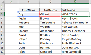
Figure 3-1: Joining first and last names.

How it works

This example illustrates the use of the ampersand (&) operator. The ampersand operator tells Excel to concatenate values with one another. As you can see in Figure 3-1, you can join cell values with text of your own. In this example, you join the values in cells B3 and C3, separated by a space (created by entering a space in quotes).

Excel also provides a CONCATENATE function that joins values without the need for the ampersand. In this example, you could enter =CONCATENATE(B3," ",C3). Frankly, it’s better to skip this function and simply use the ampersands. This function is more processing intensive and requires using more keystrokes.

Formula 14: Setting Text to Sentence Case

Excel provides three useful functions to change the text to upper-, lower-, or proper case. As you can see in rows 6, 7, and 8 illustrated in Figure 3-2, these functions require nothing more than a pointer to the text you want converted. As you might guess, the UPPER function converts text to all uppercase, the LOWER function converts text to all lowercase, and the PROPER function converts text to title case (the first letter of every word is capitalized).

What Excel lacks is a function to convert text to sentence case (only the first letter of the first word is capitalized). But as you can see in Figure 3-2, you can use the following formula to force text into sentence case:

=UPPER(LEFT(C4,1)) & LOWER(RIGHT(C4,LEN(C4)-1))

Figure 3-2: Converting text into uppercase, lowercase, proper case, and sentence case.

How it works

If you take a look at this formula closely, you can see that it’s made up of two parts that are joined by the ampersand.

The first part uses Excel’s LEFT function:

UPPER(LEFT(C4,1))

The LEFT function allows you to extract a given number of characters from the left of a given text string. The LEFT function requires two arguments: the text string you are evaluating and the number of characters you need extracted from the left of the text string. In this example, you extract the left 1 character from the text in cell C4. You then make it uppercase by wrapping it in the UPPER function.

The second part is a bit trickier. Here, you use the Excel RIGHT function:

LOWER(RIGHT(C4,LEN(C4)-1))

Like the LEFT function, the RIGHT function requires two arguments: the text you are evaluating, and the number of characters you need extracted from the right of the text string. In this case, however, you can’t just give the RIGHT function a hard-coded number for the second argument. You have to calculate that number by subtracting 1 from the entire length of the text string. You subtract 1 to account for the first character that is already uppercase thanks to the first part of the formula.

You use the LEN function to get the entire length of the text string. You subtract 1 from that, which gives you the number of characters needed for the RIGHT function.

You can finally pass the formula you’ve created so far to the LOWER function to make everything but the first character lowercase.

Joining the two parts together gives results in sentence case:

=UPPER(LEFT(C4,1)) & LOWER(RIGHT(C4,LEN(C4)-1))

Formula 15: Removing Spaces from a Text String

If you pull data in from external databases and legacy systems, you will no doubt encounter text that contains extra spaces. Sometimes these extra spaces are found at the beginning of the text, whereas at other times, they show up at the end.

Extra spaces are generally evil because they can cause problems in lookup formulas, charting, column sizing, and printing.

Figure 3-3 illustrates how you can remove superfluous spaces by using the TRIM function.

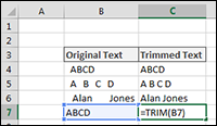
Figure 3-3: Removing excess spaces from text.

How it works

The TRIM function is relatively straightforward. Simply give it some text and it removes all spaces from the text except for single spaces between words.

As with other functions, you can nest the TRIM function in other functions to clean up your text while applying some other manipulation. For instance, the following function trims the text in cell A1 and converts it to uppercase all in one step:

=UPPER(TRIM(A1))

The TRIM function was designed to trim only the ASCII space character from text. The ASCII space character has a code value of 32. The Unicode character set, however, has an additional space character called the nonbreaking space character. This character is commonly used in web pages and has the Unicode value of 160.

The TRIM function is designed to handle only CHAR(32) space characters. It cannot, by itself, handle CHAR(160) space characters. To handle this kind of space, you need to use the SUBSTITUTE function to find CHAR(160) space characters and replace them with CHAR(32) space characters so that the TRIM function can fix them. You can accomplish this task all at one time with the following formula:

=TRIM(SUBSTITUTE(A4,CHAR(160),CHAR(32)))

For a detailed look at the SUBSTITUTE function, see Formula 18: Substituting Text Strings.

Formula 16: Extract Parts of a Text String

One of the most important techniques for manipulating text in Excel is the capability to extract specific portions of text. Using Excel’s LEFT, RIGHT, and MID functions, you can perform tasks such as:

• Convert nine-digit postal codes into five-digit postal codes
• Extract phone numbers without the area code
• Extract parts of employee or job codes for use somewhere else

Figure 3-4 demonstrates how using the LEFT, RIGHT, and MID functions can help easily accomplish these tasks.

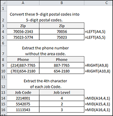
Figure 3-4: Using the LEFT, RIGHT, and MID functions.

How it works

The LEFT function allows you to extract a given number of characters from the left of a given text string. The LEFT function requires two arguments: the text string you are evaluating and the number of characters you need extracted from the left of the text string. In the example, you extract the left five characters from the value in Cell A4.

=LEFT(A4,5)

The RIGHT function allows you to extract a given number of characters from the right of a given text string. The RIGHT function requires two arguments: the text string you are evaluating and the number of characters you need extracted from the right of the text string. In the example, you extract the right eight characters from the value in Cell A9.

=RIGHT(A9,8)

The MID function allows you to extract a given number of characters from the middle of a given text string. The MID function requires three arguments: the text string you are evaluating; the character position in the text string from where to start extracting; and the number of characters you need extracted. In the example, you start at the fourth character in the text string and extract one character.

=MID(A14,4,1)

Formula 17: Finding a Particular Character in a Text String

Excel’s LEFT, RIGHT, and MID functions work great for extracting text, but only if you know the exact position of the characters you are targeting. What do you do when you don’t know exactly where to start the extraction? For example, if you had the following list of Product codes, how would you go about extracting all the text after the hyphen?

• PRT-432
• COPR-6758
• SVCCALL-58574

The LEFT function wouldn’t work because you need the right few characters. The RIGHT function alone won’t work because you need to tell it exactly how many characters to extract from the right of the text string. Any number you give will pull either too many or too few characters from the text. The MID function alone won’t work because you need to tell it exactly where in the text to start extracting. Again, any number you give will pull either too many or too few characters from the text.

The reality is that you often will need to the find specific characters in order to get the appropriate starting position for extraction.

This is where Excel’s FIND function comes in handy. With the FIND function, you can get the position number of a particular character and use that character position in other operations.

In the example shown in Figure 3-5, you use the FIND function in conjunction with the MID function to extract the middle numbers from a list of product codes. As you can see from the formula, you find the position of the hyphen and use that position number to feed the MID function.

=MID(B3,FIND("-",B3)+1,2)

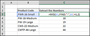
Figure 3-5: Using the FIND function to extract data based on the position of the hyphen.

How it works

The FIND function has two required arguments. The first argument is the text you want to find. The second argument is the text you want to search. By default, the FIND function returns the position number of the character you are trying to find. If the text you are searching contains more than one of your search characters, the FIND function returns the position number of the first encounter.

For instance, the following formula searches for a hyphen in the text string “PWR-16-Small”. The result will be a number 4, because the first hyphen it encounters is the fourth character in the text string.

=FIND("-","PWR-16-Small")

You can use the FIND function as an argument in a MID function to extract a set number of characters after the position number returned by the FIND function.

Entering this formula in a cell will give you the two numbers after the first hyphen found in the text. Note the +1 in the formula. Including +1 ensures that you move over one character to get to the text after the hyphen.

=MID("PWR-16-Small", FIND("-","PWR-16-Small")+1, 2)

Alternative: Finding the second instance of a character

By default, the FIND function returns the position number of the first instance of the character you are searching for. If you want the position number of the second instance, you can use the optional Start_Num argument. This argument lets you specify the character position in the text string to start the search.

For example, the following formula returns the position number of the second hyphen because you tell the FIND function to start searching at position 5 (after the first hyphen).

=FIND("-","PWR-16-Small", 5)

To use this formula dynamically (that is, without knowing where to start the search) you can nest a FIND function as the Start_Num argument in another FIND function. You can enter this formula into Excel to get the position number of the second hyphen.

=FIND("-","PWR-16-Small", FIND("-","PWR-16-Small")+1)

Figure 3-6 demonstrates a real-world example of this concept. Here, you extract the size attribute from the product code by finding the second instance of the hyphen and using that position number as the starting point in the MID function. The formula shown in cell C3 is as follows:

=MID(B3,FIND("-",B3,FIND("-",B3)+1)+1,10000)

This formula tells Excel to find the position number of the second hyphen, move over one character, and then extract the next 10,000 characters. Of course, there aren’t 10,000 characters, but using a large number like that ensures that everything after the second hyphen is pulled.

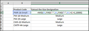
Figure 3-6: Nesting the FIND function to extract everything after the second hyphen.

Formula 18: Substituting Text Strings

In some situations, it’s helpful to substitute some text with other text. One such case is when you encounter the annoying apostrophe S (’S) quirk that you get with the PROPER function. To see what we mean, enter this formula into Excel:

=PROPER("STAR'S COFFEE")

This formula is meant to convert the given text into title case (where the first letter of every word is capitalized). The actual result of the formula is the following:

• Star'S Coffee

Note how the PROPER function capitalizes the S after the apostrophe. Annoying, to say the least.

However, with a little help from the Excel’s SUBSTITUTE function, you can avoid this annoyance. Figure 3-7 shows the fix using the following formula:

=SUBSTITUTE(PROPER(SUBSTITUTE(B4,"'","qzx")),"qzx","'")

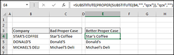
Figure 3-7: Fixing the apostrophe S issue with the SUBSTITUTE function.

How it works

The formula uses the SUBSTITUTE function, which requires three arguments: the target text; the old text you want replaced; and the new text to use as the replacement.

As you look at the full formula, note that it uses two SUBSTITUTE functions. This formula is actually two formulas (one nested in the other). The first formula is the part that reads

PROPER(SUBSTITUTE(B4,"'","qzx"))

In this part, you use the SUBSTITUTE function to replace the apostrophe (’) with qzx. This may seem like a crazy thing to do, but there is some method here. Essentially, the PROPER function capitalizes any letter coming directly after a symbol. You trick the PROPER function by substituting the apostrophe with a benign set of letters that are unlikely to be strung together in the original text.

The second formula actually wraps the first. This formula substitutes the benign qzx with an apostrophe.

=SUBSTITUTE(PROPER(SUBSTITUTE(B4,"'","qzx")),"qzx","'")

So the entire formula replaces the apostrophe with qzx, performs the PROPER function, and then reverts the qzx back to an apostrophe.

Formula 19: Counting Specific Characters in a Cell

A useful trick is to be able to count the number of times a specific character exists in a text string. The technique for doing this in Excel is a bit clever. To figure out, for example, how many times the letter s appears in the word Mississippi, you can count them by hand, of course, but systematically, you can follow these general steps:

1. Measure the character length of the word Mississippi (11 characters).
2. Measure the character length after removing every letter s (6 characters).
3. Subtract the adjusted length from the original length.

You can then accurately conclude that the number of times the letter s appears in the word Mississippi is four.

A real-world use for this technique of counting specific characters is to calculate a word count in Excel. Figure 3-8 shows the following formula being used to count the number of words entered in cell B4:

=LEN(B4)-LEN(SUBSTITUTE(B4," ",""))+1

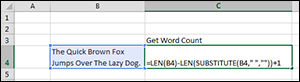
Figure 3-8: Calculating the number of words in a cell.

How it works

This formula essentially follows the steps mentioned earlier in this section. The formula uses the LEN function to first measure the length of the text in cell B4:

LEN(B4)

It then uses the SUBSTITUTE function to remove the spaces from the text:

SUBSTITUTE(B4," ","")

Wrapping that SUBSTITUTE function in a LEN function gives you the length of the text without the spaces. Note that you have to add one to that answer to account for the fact that the last word doesn’t have an associated space.

LEN(SUBSTITUTE(B4," ",""))+1

Subtracting the original length with the adjusted length gives you the word count.

=LEN(B4)-LEN(SUBSTITUTE(B4," ",""))+1

Formula 20: Adding a Line Break within a Formula

When creating charts in Excel, it’s sometimes useful to force line breaks for the purpose of composing better visualizations. Take the chart shown in Figure 3-9, for example. Here, the X-axis labels in the chart include the data value in addition to the sales rep. This setup works well when you don’t want to inundate your chart with data labels.

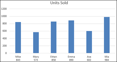
Figure 3-9: The X-axis labels in this chart include a line break and a reference to the data values.

The secret to this trick is to use the CHAR() function in a formula that makes up your chart labels (see Figure 3-10).

Figure 3-10: Using the CHAR() function to force a line break between sales rep name and data value.

How it works

Every character in Excel has an associated ANSI character code. The ANSI character code is a Windows system code set that defines the characters you see on your screen. The ANSI character set consists of 255 characters, numbered from 1 to 255. The uppercase letter A is character number 97. The number 9 is character 57.

Even nonprinting characters have codes. The code for a space is 32. The code for a line break is 10.

You can call up any character in a formula by using the CHAR() function. The example shown in Figure 3-10 calls up the line break character and joins it with the values in cells A3 and C3:

=A3 & CHAR(10) & C3

The cell itself doesn’t show the line break unless you have wrap text applied. But even if you don’t, any chart using this kind of formula will display the data returned by the formula with the line breaks.

Formula 21: Cleaning Strange Characters from Text Fields

When you import data from an external data source such as text files or web feeds, strange characters may come in with your data. Instead of trying to clean these manually, you can use Excel’s CLEAN function (see Figure 3-11).

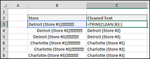
Figure 3-11: Cleaning data with the CLEAN function.

How it works

The CLEAN function removes nonprintable characters from any text you pass to it. You can wrap the CLEAN function within the TRIM function to remove unprintable characters and excess spaces at the same time.

=TRIM(CLEAN(B3))

Formula 22: Padding Numbers with Zeros

In many cases, the work you do in Excel ends up in other database systems within the organization you’re involved with. Those database systems often have field-length requirements that mandate a certain number of characters. A common technique for ensuring that a field is made up of a set number of characters is to pad data with zeros.

Padding data with zeros is a relatively easy concept to apply. Essentially, if you have a Customer ID field that must be 10 characters long, for example, you need to add enough zeros to fulfill that requirement. So Customer ID 5381656 would need to be padded with three zeros, making that ID 5381565000.

Cell C4 shown in Figure 3-12 uses this formula to pad the Customer IDs with zeros:

=LEFT(B4&"0000000000", 10)

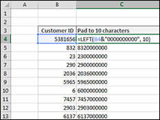
Figure 3-12: Padding Customer IDs to 10 characters.

How it works

The formula shown in Figure 3-12 first joins the value in cell B4 and a text string comprising of 10 zeros, effectively creating a new text string that guarantees a Customer ID composed of 10 zeros.

You then use the LEFT function to extract the left 10 characters of that new text string. The result will be a Customer ID with a minimum of 10 characters.

For more details on the LEFT function, see Formula 16: Extract Parts of a Text String.

Formula 23: Formatting the Numbers in a Text String

It’s not uncommon to have reporting that joins text with numbers. For example, you may be required to show a line in your report that summarizes a salesperson’s results, like this:

John Hutchison: $5,000

The problem is that when you join numbers in a text string, the number formatting does not follow. Take a look at Figure 3-13 as an example. Note how the numbers in the joined strings (column E) do not adopt the formatting from the source cells (column C).

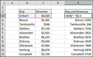
Figure 3-13: Numbers joined with text do not inherently adopt number formatting.

To solve this problem, you have to wrap the cell reference for your number value in the TEXT function. Using the TEXT function, you can apply the needed formatting on the fly. The formula shown in Figure 3-14 resolves the issue:

=B3&": "&TEXT(C3, "$0,000")

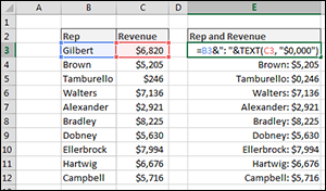
Figure 3-14: Using the TEXT function allows you to format numbers joined with text.

How it works

The TEXT function requires two arguments: a value, and a valid Excel format. You can apply any formatting you want to a number as long as it’s a format that Excel recognizes.

For example, you can enter this formula into Excel to display $99:

=TEXT(99.21,"$#,###")

You can enter this formula into Excel to display 9921%:

=TEXT(99.21,"0%")

You can enter this formula into Excel to display 99.2:

=TEXT(99.21,"0.0")

An easy way to get the syntax for a particular number format is to look at the Number Format dialog box. To see that dialog box and get the syntax, follow these steps:

1. Right-click any cell and select Format Cell.
2. On the Number format tab, select the formatting you need.
3. Select Custom from the Category list on the left of the Number Format dialog box.
4. Copy the syntax found in the Type input box.

Alternative: Using the DOLLAR function

If the number value you’re joining with text is a dollar figure, you can use the simpler DOLLAR function. This function applies the regional currency format to the given text.

The DOLLAR function has two basic arguments: the number value and the number of decimals you want to display.

=B3&": "&DOLLAR(C3,0)