3.1 Models
In this chapter, we introduce the concept of model, essential point of statistical inference. The concept is reviewed here by our algebraic interpretation. The general definition is very simple:
Definition 3.1.1
A model on a system S of random variables is a subset M of the space of distributions  .
.
Of course, in its total generality, the previous definition it is not so significant.
The Algebraic Statistics consists of practice in focus only on certain particular types of models.
Definition 3.1.2
A model M
on a system S is called algebraic model
if, in the coordinates of  , M corresponds to the set of solutions of a finite system of polynomial equations. If the polynomials are homogeneous, then M si called a homogeneous algebraic model.
It occurs that the algebraic models are those mainly studied by the proper methods of Algebra and Algebraic Geometry.
In the statistical reality, it occurs that many models, which are important for the study of stochastic systems (discrete), are actually algebraic models.
Example 3.1.3
On a system S, the set of distributions with constant sampling is a model M. Such a model is a homogeneous algebraic one.
 are the random variables in S and we identify
  with
with  , where the coordinates are
  , then M is defined by the homogeneous equations:
3.2 Independence Models
The most famous class of algebraic models is the one given by independence models. Given a system S, the independence model on S is, in effect, a subset of the space of distributions of the total correlation  , containing the distributions in which the variables are independent among them. The basic example is Example 2.3.13, where we consider a Boolean system S, whose two variables x, y represent, respectively, the administration of the drug and the healing.
This example justifies the definition of a model of independence, for the random systems with two variables (dipoles) , already in fact introduced in the previous chapters.
Definition 3.2.1
Let S be a system with two random variables  and let
  . The space of
  distributions on T is identified with the space of matrices
  , where
  is the number of states of the variable
  .
.
We recall that a distribution  is a distribution of independence if D, as matrix, has rank
  .
.
The independence model on S is the subset of  of distributions of rank
  .
.
To extend the definition of independence to systems with more variables, consider the following example.
Example 3.2.2
Let S be a random system, having three random variables  representing, respectively, a die and two coins (this time not loaded). Let
  and consider the
  -distribution D on T defined by the tensor
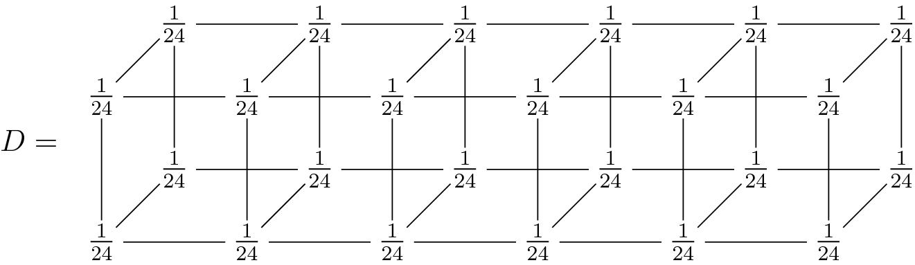
It is clear that D is a distribution of independence and probabilistic. You can read it like the fact that the probability that a d comes out from the die at the same time of the faces (for example, T and H) from the two coins, is the product of the probability  that d comes out of the die times the probability
  that T comes out of the coin times the probability
  that H comes out of the other coin.
Hence, we can use Definition 6.3.3 to define the independence model.
Definition 3.2.3
Let S be a system with random variables  and let
  . The space of K-distributions on T is identified with the space of tensors
  , where
  is the number of states of the variable
  .
.
A distribution  is a distribution of independence
if D lies in the image of independence connection (see Definition 2.3.4), i.e., as a tensor, it has rank 1 (see Definition 6.3.3).
is a distribution of independence
if D lies in the image of independence connection (see Definition 2.3.4), i.e., as a tensor, it has rank 1 (see Definition 6.3.3).
The independence model
on X is the subset of  consisting of all distributions of independence (that is, of all tensors of rank 1).
The model of independence, therefore, corresponds to the subset of simple (or decomposable) tensors in a tensor space (see Remark 6.3.4).
We have seen, in Theorem 6.4.13 of the chapter on Tensorial Algebra, how such subset can be described. Since all relations (6.4.1) correspond to the vanishing of one (quadratic) polynomial expression in the coefficients of the tensor, we have
Corollary 3.2.4
The model of independence is an algebraic model.
Note that for the tensors  , the independence model is defined by 12 quadratic equations (6 faces + 6 diagonal).
The equations corresponding to the equalities (6.4.1) describe a set of equations for the model of independence. However such a set, in general, it is not minimal.
The distributions of independence represent situations in which there is no link between the behavior of the various random variables of S, which are, therefore, independent.
There are, of course, intermediate cases between a total link and a null link, as seen in the following:
Example 3.2.5
 consists of tensors of dimension 3 and type
  . We say that a distribution
  is without triple correlation
if there exist three matrices
is without triple correlation
if there exist three matrices  ,
,  ,
,  such that for all i, j, k:


3.3 Connections and Parametric Models
Another important example of models in Algebraic Statistics is provided by the parametric models. They are models whose elements have coefficients that vary according to certain parameters. To be able to define parametric models, it is necessary first to fix the concept of connection between two random systems.
Definition 3.3.1
Let S, T be system of random variables. We call K-connection between S and T any function  from the space of K-distributions
  to the space of K-distributions
  .
.
As usual, when the field K is understood, we will omit it in the notation.
After all, therefore, connections are nothing more than functions between a space  and a space
  . The name we gave, in reference to the fact that these are two spaces connected to random systems, serves to emphasize the use we will make of connections: to transport distributions from the system S to the system T.
In this regard, if T has n random variables  , and the alphabet of each variable
  has
has  elements, then
  can be identified with
  . In this case, it is sometimes useful to think of a connection
  as a set of functions
  .
.
 are all possible states of the variables in S, and
  are the possible states of the variable
  , then we will also write
 functions; not even continuity. Of course, in concrete cases, we will study in particular certain connections having well-defined properties.
It is clear that, in the absence of any property, we cannot hope that the more general connections satisfy many properties.
Let us look at some significant examples of connections.
Example 3.3.2
Let S be a random system and  a subsystem of S. You get a connection from S to
  , called projection simply by forgetting the components of the distributions which correspond to random variables not contained in
  .
.
Example 3.3.3
 its total correlation. Assume that S has random variables
  , and each variable
  has
has  states, then
  is identified with
  . In Definition 2.3.4, we defined a connection
  , called connection of independence
or Segre connection, in the following way:
, called connection of independence
or Segre connection, in the following way:  sends the distribution
 )
)  such that
 .
.Clearly there are other interesting types of connection. A practical example is the following:
Example 3.3.4
Consider a population of microorganisms in which we have elements of two types, A, B, that can pair together randomly. In the end of the couplings, we will have microorganisms with genera of type AA or BB, or mixed type  .
.
The initial situation corresponds to a Boolean system with a variable (the initial type  ) which assumes the values A, B. At the end, we still have a system with only one variable (the final type t) that can assume the 3 values AA, AB, BB.
If we initially insert a distribution with  elements of type A and
  elements of type B, which distribution we can expect on the final variable t?
An individual has a chance to meet another individual of type A or B which is proportional to (a, b), then the final distribution on t will be  given by
  ,
,  ,
,  . This procedure corresponds to the connection
 .
.
Definition 3.3.5
We say that a model  is parametric if there exists a random system S and a connection
  from S to T such that V is the image of S under
  in
in  , i.e.,
  .
.
A model is polynomial parametric if  is defined by polynomials.
A model is toric
if  is defined by monomials.
 are all possible states of the variables in S, and
  are the possible states of the variables
  of T, then in the parametric model defined by the connection
  we have
 ’s represent the components of
  .
.The model definition we initially gave is so vast to be generally poorly usable. In reality, the models we will use in the following will always be algebraic models or polynomial parametric.
Example 3.3.6
It is clear from the Example 3.3.3 that the model of independence is given by the image of the independence connection, defined by the Segre map (see the Definition 10.5.9), so it is a parametric model.

From its parametric equations, (3.3.1), we quickly realize that the independence model is a toric model.
Example 3.3.7

Remark 3.3.8
It is evident, but it is good to underline it, that for the definitions we gave, being an algebraic or polynomial parametric model is independent from changes in coordinates. Being a toric model instead it can depend on the choice of coordinates.
Definition 3.3.9
The term linear model
denotes, in general, a model on S defined in  by linear equations.
Obviously, every linear model is algebraic and also polynomial parametric, because you can always parametrize a linear space.
Example 3.3.10
Even if a connection  , between the K-distributions of two random systems S and T, is defined by polynomials, the polynomial parametric model that
  defines it is not necessarily algebraic!.
In fact, if we consider  and two random systems S and T each having one single random variable with a single state, the connection
  ,
,  certainly determines a polynomial parametric model (even toric) which corresponds to
  , so it can not be defined in
  as vanishing of polynomials.
We will see, however, that by widening the field of definition of distributions, as we will do in the next chapter switching to distributions on  , under a certain point of view all polynomial parametric models will, in fact, be algebraic models.
The following counterexample is a milestone in the development of so much part of the Modern mathematics. Unlike Example 3.3.10, it cannot be recovered by enlarging our field of action.
Example 3.3.11
Not all algebraic models are polynomial parametric.
We consider in fact a random system S with only one variable having three states. In the distribution space  , we consider the algebraic model V defined by the unique equation
  .
.
There cannot be a polynomial connection  from a system
  to S whose image is V.
In fact, suppose the existence of three polynomials p, q, r, such that  . Obviously, the three polynomials must satisfy identically the equation
  . It is enough to verify that there are no three polynomials satisfying the previous relationship. Provided to set values for the other variables, we can assume that p, q, r are polynomials in a single variable t. We can also suppose that the three polynomials do not have common factors. Let us say that
  .
.


 must be proportional to the
  -minors of the matrix, hence
  is proportional to
  , and so on. Considering the equality
  , we get that
  divides
  , hence
  which contradicts the fact that
  .
.Naturally, there are examples of models that arise from connections that they do not relate a system and its total correlation.
Example 3.3.12
Let us say we have a bacterial culture in which we insert bacteria corresponding to two types of genome, which we will call A, B.
Suppose, according to the genetic makeup, the bacteria can develop characteristics concerning the thickness of the membrane and of the core. To simplify, let us say that in this example, cells can develop nucleus and membrane large or small.
According to the theory to be verified, the cells of type A develop, in the descent, a thick membrane in  of cases and develop large core in
  of cases. Cells of type B develop thick membrane in the
  of cases and a large core in one-third of the cases. Moreover, the theory expects that the two phenomena are independent, in the intuitive sense that developing a thick membrane is not influenced by, nor influences, the development of a large core.
We build two random systems. The first S, which is Boolean, has only one variable random c (= cell) with A, B states. The second T with two boolean variables, m (= membrane) and n (= core). We denote for both with 0 the status “big” and with 1 the status “small”.
 between S and T. In the four states of the two variables of T, which we will indicate with
  , this connection is defined by
 .
.
 : indicating with
  the variables corresponding to the four states of the only variable of
  , then such connection
  is defined by
 :
:
 of cells with a thick membrane, nucleus, etc.
In the real world, of course, some tolerance should be expected from experimental data error. The control of this experimental tolerance will be not addressed in this book, as it is a part of standard statistical theories.
3.4 Toric Models and Exponential Matrices
Recall that a toric model is a parametric model on a system T corresponding to a connection from S to T which is defined by monomials.
Definition 3.4.1
Let W be a toric model defined by a connection  from S to T. Let
  be all possible states of all the variables of S and let
  the states of all the variables of T. One has, for every i,
  , where each
  is a monomial in the
  .
.
We will call exponential matrix
of W the matrix  , where
  is the exponent of
  in
in  .
.
E is, therefore, a  array of nonnegative integers. We will call it complex associated with W the subset of
  formed by the points corresponding to the rows of E.
Proposition 3.4.2
Let W be a toric model defined by a monomial connection  from S to T and let E be its exponential matrix.
Each linear relationship  among the
  rows of E corresponds to implicit polynomial equations that are satisfied by all points in W.
Proof
 among the rows of E. We associate to this relation a polynomial equation
 the monomial coefficient,
In effect, by replacing  with their expressions in terms of
  , we get two monomials with equal exponents and opposite coefficients, which are canceled.
Note that the polynomial equations obtained previously, are in fact binomial.
Definition 3.4.3
The polynomial equations associated with the linear relations between the rows of the exponential matrix of a toric model W define an algebraic model containing W. This model takes the name of algebraic model generated by W.
It is clear from Example 3.3.10 that the algebraic model generated by a toric model W always contains W, but it does not always coincide with W. Let us see a couple of examples about it.
Example 3.4.4
We still consider the example of the model of independence on a dipole S.
 the states of the first variable T and with
  the states of the second variable. The resulting model is parametrically defined, on
  , by
, by  . It is, therefore, a toric model, whose exponential matrix is given by

 , exactly the
  -minors of the matrices in the model.
It follows that the algebraic model associated to this connection coincides with the space of matrices of rank  , which is exactly the image of the connection of independence.
Example 3.4.5
 given by the parametric equations

 . Using the formula for the coefficients, we get the equation in
  :
:
 defined by this equation does not coincide with W. As a matter of fact, it is clear that the points in W have nonnegative x, z, while the point
  is in
is in  .
.However, one has  where B is the subset of the points in
  with nonnegative coordinates. In fact, if (x, y, z) is a point in B which satisfies the equation, then, posing
  ,
,  , one has
  .
.
Remark 3.4.6
The scientific method.
Given a parametric model, defined by a connection  from S to T, if we know an “initial” distribution D over S (the experiment data) and we measure the distribution
  that we derive on T (the result of the experiment), we can easily deduce if the hypothesized model fits or not with reality.
But if we have no way of knowing the D distribution and we can only measure the  distribution, as happens in many real cases, then it would be a great help to know some polynomial F that vanishes on the model, that is, to know its implicit equations. In fact, in this case the simple check of the fact that
  can give us many indications: if the vanishing does not occur, our model is clearly inadequate; instead if it occurs, it gives a clue in favor of the validity of the model.
If we then knew that the model is also algebraic and we knew the equations, their control over many distributions, results of experiments, would give a good scientific evidence on the validity of the model itself.