). We can read this out loud as “yields,” “proves,” or “therefore.” We can read the expression
When we make an argument, we might “feel certain” about our reasoning, but in formal logic that’s not good enough. We must produce a rigorous case that demonstrates why we can’t be wrong, and we must formally prove our case to someone else. That’s a tall order! If we really want to be sure about the validity of an argument, we need to write it down in a way that eliminates potential “gaps” between the steps, while at the same time maintaining clear language. We call this sure-fire way of expressing an argument a formal system or formal logic. The simplest way to learn proofs involves a formal system called propositional logic, also known as sentential logic, the propositional calculus, or the sentential calculus. Propositional and sentential refer to our subject matter, which comprises sentences. In logic, the term calculus doesn’t refer to the mathematical discipline involving graphs and changing quantities; it reminds us that we can “calculate” proofs in a formal system of reasoning.
CHAPTER OBJECTIVES
In this chapter, you will
• String symbols together to construct propositional formulas.
• Learn the structural rules for sequents and arguments.
• Manipulate expressions containing logical operations.
• Apply fundamental laws of logic to prove simple theorems.
• Discover how to prove a theorem by deriving a contradiction.
To make a formal system in logic, we use symbols—a “logical language” without any of the subtle meanings and complicated grammar that make absolute certainty so hard to achieve in everyday speech. Because of the special logical language, some people call this system symbolic logic. Each symbol has only one meaning, and rules exist that tell us how we can use it. We can “translate” our arguments from English into the system when we want to prove something about them. We call the resulting string of symbols a formula.
We’ve been talking about sentences, but we haven’t asked the basic question: What counts as a sentence in propositional logic? We can think of formulas made up of the symbols we have introduced that constitute mere gibberish, and that don’t represent a definite proposition at all. Some examples follow:
)PQ(¬
)P ∧ Q(∨ (R)
(P ∧ ↔ Q
Any string of “approved” symbols technically constitutes a formula, but it only expresses logical relationships when it follows the rules of syntax suggested as we introduced them. The formulas above don’t express propositions, so we wouldn’t know where to start assigning them truth values based on their variables. A formula that follows the rules (like most you’ll encounter) is called a propositional formula (PF), propositional expression, or sentential formula.
Let’s recap our syntax rules to give a rigorous definition of what qualifies as a PF in the formal system we have set up:
• Any propositional variable (symbolized by a capital letter) is a PF.
• Any PF preceded by the symbol ¬ is a PF. For example, if X is a PF, then ¬X is a PF.
• Any PF joined by one of the symbols ∧, ∨, → or ↔ (known as binary connectives because they join together two propositions) to another PF, the whole thing inside parentheses, constitutes a PF. For example, if X is a PF, Y is a PF, and # is a binary connective, then (X # Y) is a PF.
• Any formula that does not satisfy at least one of the three conditions listed above does not constitute a PF.
All PFs constructed according to these rules include parentheses around everything but atomic propositions, including the whole formula as written. Too many parentheses can clutter a formula, so you can “drop” parentheses according to the established order of operations as an “informal” (but always unambiguous) shorthand. You can substitute the parentheses back in at any time to satisfy the strict definition of a PF above. Dropping unnecessary parentheses sometimes makes PFs appear simpler. You can use extra parentheses whenever you think that doing so will ensure that your reader correctly understands the formula.
We’re using operators, variables, and formulas set off by parentheses in our formal system. If this notation reminds you of a course in mathematics, your hunch is well founded! Many of the conventions of formal logic were created with mathematics in mind. In fact, some people call symbolic logic mathematical logic. This doesn’t mean propositional logic has anything to do with polygons or rational numbers, just that we want to achieve the same kind of rigor and certainty here that mathematicians use in, say, a proof in Euclidean geometry.
Some of our rules will involve the idea of a logical contradiction. This means what you might expect: a statement that disagrees with itself and therefore can’t possibly hold true as a whole. We can’t talk about contradiction in the everyday sense, though; we have to assign it a rigorous formal meaning that makes it as certain as the rest of the system.
Let C represent the sentence “It’s cold outside,” and let H represent the sentence “It’s hot outside.” You might at first think that the conjunction C ∧ H constitutes a contradiction, but it really doesn’t! We could disagree about the cutoff points for what we consider “hot” or “cold.” We might define “in-between” states such as “warm”; this means that H does not negate C, strictly speaking. If we are to call a proposition a formal contradiction, that proposition must constitute the conjunction of a sentence with its own exact negation, as in C ∧ ¬C. Then we have no room for error; ¬C always has the opposite truth value from C, so we know for sure that one will be true and the other false (even though we might not know which is which). If we say “It’s cold and it’s not cold” or “It’s hot and it’s not hot,” then we state a logical contradiction in the strictest formal sense.
Any argument that we can prove in our system can be understood as a sequent, which means that we can summarize it as the set of propositions that act as premises and the single proposition that we prove from them. We will express all of our propositions as PFs, and we will divide the premises from the conclusions using a symbol called a tee, a turnstile, or an assertion sign (). We can read this out loud as “yields,” “proves,” or “therefore.” We can read the expression
P ∧ Q Q
as “P and Q, therefore Q.” We can also say that Q is derivable from P and Q. The assumption set on the left side is sometimes called the antecedent, and the conclusion on the right is called the succedent. (Be careful—the first part of a conditional proposition is also called an antecedent.) When we have multiple propositions in the antecedent, we’ll separate them with commas, as we would do when writing a list; for example,
Q, R Q ∧ R
The order of the premises doesn’t matter; we could have listed the premises in the last sequent as R, Q without producing a different sequent (and without changing the corresponding proof).
 Still Struggling
We use the designation sequent expression because a written sequent does not constitute a PF or a proposition. Accordingly, does not constitute a symbol of our formal language. As with truth assignments (and truth tables), we use sequents to talk about statements that constitute a part of the logical language, rather than to make statements within the language. The language that we use to discuss the propositional calculus, consisting of symbols and conventions used in this way, is called the logical metalanguage.
The purpose of having a logical system is to facilitate proofs of propositions without leaving anything to the imagination, so we always get valid results. Logicians have a formal way of writing down one proposition after another according to specific rules, and it gives anyone reading it all the pieces they need to follow the argument.
We write the sequent that we want to prove first; then we put down the propositions in our argument line by line beneath that initial sequent, expressing them all as PFs. In addition to the proposition itself, every line should include a line number for reference (on the left), a rule justifying the assertion, references showing how the rule fits in with the previous lines of the proof, and a tally of assumptions that we have employed to derive the proposition (all to the right of the PF). That gives us five columns in total. The reference column will indicate which propositions we’re talking about (using the line numbers in the reference column), and the rule column shows what kind of deduction we’re performing, using abbreviated names for the rules. This way, we can check each step of the proof for validity. We should always list the reference and assumption line numbers in numerical order.
The premise side of the sequent being proved is often introduced in the first line(s) of a proof, and the conclusion side should constitute the last line. In the assumptions column, we’ll be able to see that the final proposition derives exclusively from the assumption(s) set out in the sequent.
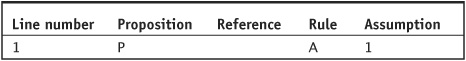
A proof usually begins with an assumption and goes from there; the corresponding rule is the most basic one in the system. As you might imagine, we never deduce our assumptions from anything. Assumptions come “out of nowhere.”
When we justify a proposition by assumption (abbreviated to an uppercase letter A), that assumption can comprise any claim we want to make, regardless of the other propositions that we’ve written down. We can introduce a proposition by assumption at any point in the proof. (We only need to make sure that the argument follows from the assumptions we’ve made—not that every assumption actually holds true in the “real world.”) We don’t have to reference any other lines from the proof as premises. We can simply write the letter A, and then put down the line number again under the assumptions column; the only assumption this line depends on is itself.
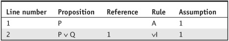
TABLE 2-1 The rule of assumption: P P.
The simplest sequent for which we can write a “proof” is the fact that if we assume a preposition P, then we assert its truth. No one would dispute the fact that this makes a valid argument (even if it’s the most trivial argument imaginable). Table 2-1 shows the formal demonstration. This constitutes a special case, because we can write the only premise and the conclusion with a single proposition, thereby proving the sequent in a single line.
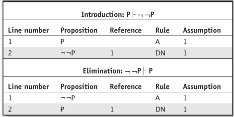
The rule of double negation allows the negation operator to be introduced and eliminated based on the idea that two instances of ¬ in a row “cancel each other out.” If someone says “It is not the case that it is not the case that it is cold outside,” she’s saying that it’s cold outside; the statement ¬¬ C is logically equivalent to the statement C.
When using the rule of double negation in a proof, you can abbreviate the rule as DN. You can use DN to add or take away pairs of negation symbols. Because DN transforms a single proposition into another logically equivalent one, you only need to reference that one line and copy over the same set of assumptions. Table 2-2 shows two simple examples.
TABLE 2-2 Two examples of double negation.
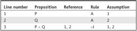
If you want to derive a ∧-statement, you can use the rule of conjunction introduction, abbreviated as ∧I. This rule lets you construct a conjunction between two propositions that you’ve already derived. Write the line numbers for the two conjuncts in the reference column and combine their assumptions. All of the premises needed to establish the conjuncts are premises of the ∧-statement. Changing the order of a ∧-statement never changes its truth value, so you can put the resulting proposition in whatever order you wish. In the example shown by Table 2-3, you could derive Q ∧ P instead of P ∧ Q by following the same steps.
TABLE 2-3 The rule of conjunction introduction: P, Q P ∧ Q.
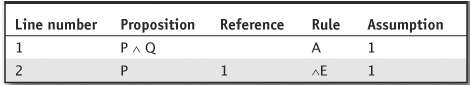
You will need a way to take apart ∧-statements as well. To do this, use the rule of conjunction elimination. This rule lets you derive the proposition on either side of the symbol ∧ by itself; the proposition will be the conjunct that you want to isolate. Cite the conjunction in the reference column, carry over all the same assumptions, and abbreviate the rule as ∧E. Just as with conjunction introduction, the order doesn’t matter in the logical sense; you can “break off” either side of the conjunction. Table 2-4 illustrates an example.
TABLE 2-4 The rule of conjunction elimination: P ∧ Q P.
You can use the rule of disjunction introduction to derive a ∨-statement on the basis of one or both of two propositions. That’s the only line you must reference; you copy over the assumptions. The rule is abbreviated as ∨I. You can “add on” the other disjunct and ∨ symbol to either side of the premise. Though it may seem strange at first glance, you can introduce any PF you want as the unreferenced disjunct without adding any new assumptions, and you’ll generate a valid deduction anyway. Table 2-5 shows an example.
TABLE 2-5 The rule of disjunction introduction: P P ∨ Q.
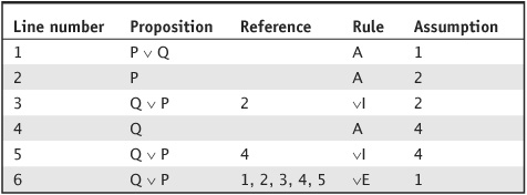
To get rid of a disjunction, you need the rule of disjunction elimination, abbreviated ∨E. This principle is a little trickier and more complex than the other inference rules that you’ve seen so far. It requires that you reference more lines. To establish that a proposition follows from a disjunction, you must prove that you can derive it from either disjunct by itself. When you want to prove something like this, you must introduce both disjuncts as assumptions, one at a time. You must therefore prove your desired conclusion twice: once following from each disjunct (along with any other assumptions that you make).
Don’t worry about taking on “extra” premises for the proof as a whole. Such assumptions are temporary. You’ll eliminate them before you finish the process. This is the first time that a rule has allowed you to “drop” an assumption, but this tactic constitutes a crucial part of doing proofs. If using assumptions provisionally and then discarding them were not allowed, you could never make any assumptions other than the premises given by the sequent.
The foregoing steps always take at least five lines to accomplish, even in the simplest case. On the line where you use the rule ∨E, you need to write five line numbers in the reference column, noting:
• The original ∨-statement
• The left-hand disjunct (as an assumption)
• The conclusion (derived from the left-hand disjunct)
• The right-hand disjunct (as an assumption)
• The conclusion (derived from the right-hand disjunct)
You should copy over all the assumptions that constitute premises for the disjunction at the start, as well as any extra assumptions (from elsewhere in the proof) that you might need to derive the conclusion along “either leg” of the argument. You use these assumptions to “test out” each disjunct as a part of the inference.
The sequence of logical steps shown in Table 2-6 uses ∨E to prove that the order of a disjunction doesn’t matter (that is, Q ∨ P follows from P ∨ Q].
TABLE 2-6 Proof of P ∨ Q Q ∨ P using disjunction elimination.
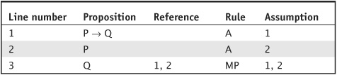
An interesting rule known as modus ponens allows you to reason with conditional propositions. If you have derived an if/then statement and its antecedent, you can prove its consequent. The name of this rule derives from the Latin modus ponendo ponens, which translates to “the way that affirms by affirming.” Let’s abbreviate it as MP (some texts use MPP). Once in awhile, you’ll hear a logician refer to the use of MP as confirming the antecedent.
You’ll need two references to make an MP inference, corresponding to the conditional proposition and its antecedent. The concluding proposition on the MP line will be the consequent of the conditional proposition. To use MP, you combine the assumptions from both of the premises to get to the logical conclusion. Table 2-7 shows how the rule works in its most basic form.
TABLE 2-7 The rule of modus ponens: P → Q, P Q.
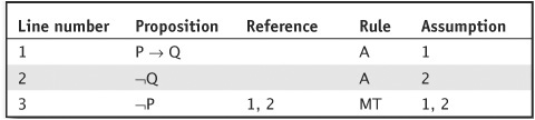
The second way to argue from a conditional statement makes use of a rule called modus tollens. The term comes from the Latin expression modus tollendo tollens, which means “the way that denies by denying.” Let’s abbreviate it as MT (some texts use MTT). You may also see this argument form referred to as denying the consequent.
The rule of MT reasons that, if you negate the consequent of a conditional statement, you “automatically” negate the antecedent as well. To demonstrate MT, you must reference two lines (the conditional statement and the negation of its consequent) and combine their assumptions, as shown in Table 2-8.
TABLE 2-8 The rule of modus tollens: P → Q, Q P.
The rule of conditional proof (abbreviated CP) introduces the → symbol. This argument form allows you to “pull out” one of your assumed premises and turn it into an antecedent, making the proposition you derived from it into the consequent.
In order to use the rule of CP, assume the truth of the statement that you want to serve as the antecedent of the conditional, and then prove the proposition that you want to serve as the consequent, using the other methods of inference you’ve learned. On the line where you employ CP, reference the premise and conclusion that you will transform into a conditional proposition. The assumptions will be the same as the ones listed for the consequent, except that you’ll drop the assumption corresponding to the antecedent. Unlike the other binary connectives, swapping the propositions from left to right (reversing the direction of the implication) makes a big difference in the meaning!
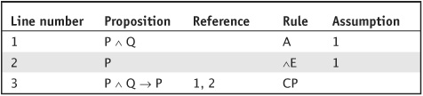
The rule of CP gives you enhanced power to get rid of superfluous assumptions. Sometimes, you can eliminate all of the assumptions from a proof! Logicians and mathematicians call a proposition that relies on no premises a theorem. The example in Table 2-9 represents the first time that we’ve seen this kind of sequent. Note that the antecedent side is blank. When reading off the symbol with no premises on the left, don’t read it as “yields,” “proves,” or “therefore.” Instead, read it as “It is a theorem that…” In evaluative terms, theorems hold true under any assignment of truth values to atomic propositions. The proof in Table 2-9 translates to the statement “It is a theorem that P ∧ Q → P.”
TABLE 2-9 The rule of conditional proof: P ∧ Q → P.
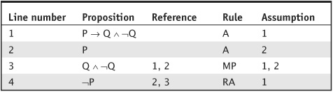
The rule of reductio ad absurdum allows you to derive a proposition by assuming its negation, and then showing that such an assumption leads to a direct contradiction (also called an absurdity)—the conjunction of some statement and its negation. The name translates from the Latin “reduction to the absurd”; we’ll abbreviate it to RA (some texts use RAA).
Assuming the “opposite” of what you want to prove might at first seem like an illogical and counterintuitive thing to do, but it works! (Alternatively, you could think of it as assuming something in order to derive its negation.) Here’s the idea: If you can derive a contradiction from a proposition, then that proposition cannot possibly hold true. If it isn’t true, then its negation must hold true.
Start off by assuming the opposite of what you’d like to prove. If you want to prove P, then you must assume ¬P. Then, employ the other derivation techniques that you’ve learned to produce a contradiction of the form Q ∨ ¬Q, where Q can be any statement whatsoever. Once you have a contradiction, you can invoke RA; because you have a contradiction, you know that (at least) one of your assumptions needs to be denied in order to be consistent. You can “blame” the contradiction on any of the assumptions used to derive it, and then you can negate it based on the remaining assumptions. Finally, you drop the negated assumption, reducing the total assumption tally by one.
TABLE 2-10 Proof of P → Q ∧ ¬Q ¬P using reductio ad absurdum.
On the line where you negate the target proposition, reference both the line where you introduced it by assumption and the line on which a contradiction appeared (with the other line listed in the assumption column). You should copy over all of the assumptions cited on the contradiction line, other than the one that you intend to negate. Table 2-10 shows an example of RA at work.
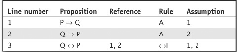
The rule of biconditional introduction says that if you can derive a conditional statement in “both directions” between two propositions, then you can put a ↔ symbol in between them. If you like, you can think of the biconditional as shorthand:
P ↔ Q means the same thing as (P → Q) ∧ (Q → P)
To introduce a biconditional operator, reference the two conditional statements that show different directions of implication between the same two propositions, and then combine their assumptions. It doesn’t matter which propositional formula (PF) you put on the left-hand side of the connective and which PF you put on the right-hand side. In proofs, you can symbolize this rule by writing ↔I. Table 2-11 illustrates ↔I in action.
TABLE 2-11 The rule of biconditional introduction: P → Q, Q → P Q ↔ P.
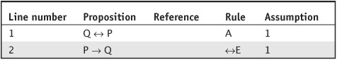
TABLE 2-12 The rule of biconditional elimination: Q ↔ P P → Q.
The rule of biconditional elimination allows you to “extract” a conditional proposition from a biconditional statement. To eliminate a biconditional operator, reference the line on which it appears and copy over the same assumptions. The result will be one of the two possible conditional statements, corresponding to one direction of implication in the original proposition. You can symbolize this rule in proofs by writing ↔E. Table 2-12 illustrates ↔E in action.
Until now, we’ve treated propositional variables mainly in the expressions of simple declarative sentences. But variables can serve as stand-ins for any proposition, so we can substitute one for another whenever we want. For example, we’ve proved that
¬¬P P
so we can go back and construct another valid proof by substituting the letter Q every time P appears. Then we end up with the derivation
¬¬Q Q
We can substitute more complex propositions, too. For example, the statement
¬¬P P
allows us to derive, using substitution, the more complex statement
¬¬(Q → R) (Q → R)
Logical arguments depend only on the form and relationships of propositions, so all arguments of this form remain valid regardless of what statements we “plug in.”
TIP From the principle of substitution, we know that we can rely on the inference rules to apply to any PF, even though we’ve only shown them for P, Q, and R. Proofs in pure logic hold true in general. But we had better watch out! If we want substitution to work, we must treat every instance in exactly the same way. If we accidentally change the form (by, say, substituting Q for some instances of P and R for other instances of P), then we lose the validity of the PF, sequent or proof.
 PROBLEM 2-1
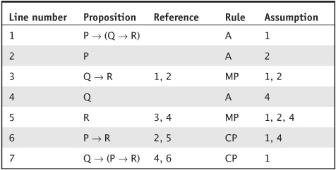
Use the inference rules to prove the sequent P → (Q → R) Q →(P → R).
 SOLUTION
See Table 2-13.
TABLE 2-13 Proof of the sequent P → (Q → R) Q → (P →R).
PROBLEM 2-2
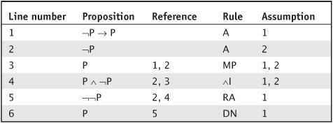
Prove the sequent ¬P → P P.
SOLUTION
See Table 2-14.
TABLE 2-14 Proof of the sequent ¬P → P P.
PROBLEM 2-3
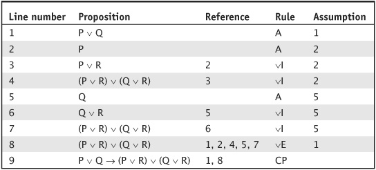
Prove the theorem P ∨ Q → (P ∨ R) ∨ (Q ∨ R).
SOLUTION
See Table 2-15.
TABLE 2-15 Proof of the theorem P ∨ Q → (P ∨ R) ∨ (Q ∨ R).
PROBLEM 2-4
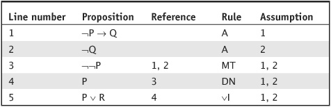
Prove the sequent ¬P → Q, ¬Q P ∨ R.
SOLUTION
See Table 2-16.
TABLE 2-16 Proof of the sequent ¬P → Q, ¬Q P ∨ R.
Logical operators obey certain rules known as laws. Several of the most basic and helpful laws of propositional logic follow. You can verify the validity of any law using a truth table. Do you recognize some of these tables from examples in the last chapter?
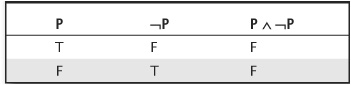
As we’ve seen already, a formal contradiction always turns out false. We call this the law of contradiction, symbolized as follows:
(P ∧ ¬P) = F
Table 2-17 illustrates the law of contradiction.
TABLE 2-17 Truth table for the law of contradiction.
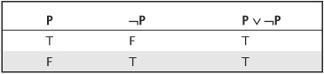
The law of excluded middle states that every proposition is either true or false. We can express this law symbolically as
(P = T) ∨ (¬P = T)
TABLE 2-18 Truth table for the law of excluded middle.
Logicians usually write it more simply as follows:
(P ∨ ¬P) = T
Table 2-18 illustrates the law of excluded middle.
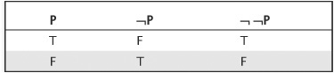
The inference rule for double negation (DN) depends on the logical equivalence of a proposition and its double-negation.
¬¬P ↔ P
Table 2-19 illustrates the law of double negation.
TABLE 2-19 Truth table for the law of double negation.
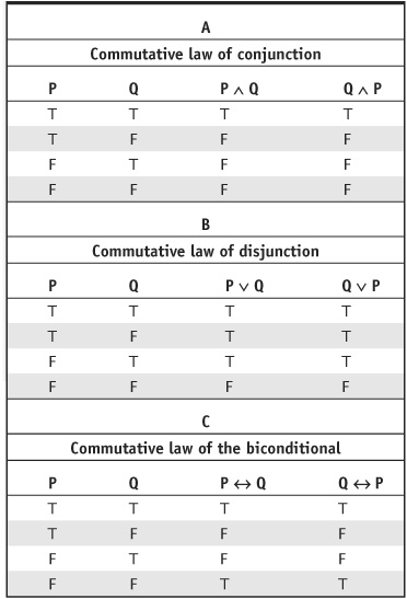
Order doesn’t matter for some operators, meaning that you can swap the propositions on both sides, and the result remains logically equivalent to the original. These properties give us the so-called commutative laws. In propositional logic, three commutative laws exist, as follows:
• Commutative law of conjunction: (P ∧ Q) ↔ (Q ∧ P)
• Commutative law of disjunction: (P ∨ Q) ↔ (Q ∨ P)
• Commutative law of the biconditional: (P ↔ Q) ↔ (Q ↔P)
TABLE 2-20 Truth tables for the commutative laws.
Tables 2-20A, 2-20B, and 2-20C verify the commutative laws of conjunction, disjunction, and the biconditional, respectively. Some logicians refer to the commutative laws as the commutative properties.
When two conjunctions join three propositions, it doesn’t matter how you group the variables. Suppose that you have the following informal PF:
P ∧ Q ∧ R
When writing in the parentheses, you can group it in either of two logically equivalent ways:
(P ∧ Q) ∧ R
or
P ∧ (Q ∧ R)
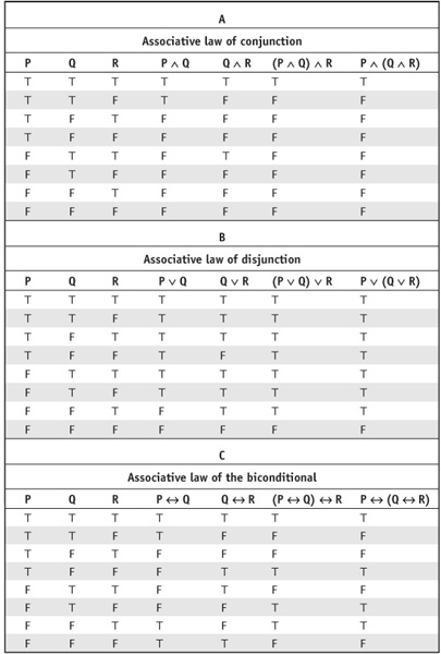
The same holds for disjunctions and biconditionals, so we have the three following associative laws.
• Associative law of conjunction: [(P ∧ Q) ∧ R] ↔ [P ∧ (Q ∧ R)]
• Associative law of disjunction: [(P ∨ Q) ∨ R] ↔ [P ∨ (Q ∨ R)]
• Associative law of the biconditional: [(P ↔ Q) ↔ R] ↔ [P ↔ (Q ↔ R)]
TIP Exercise caution with the associative laws. They only work when both operators in a three-statement PF are of the same type. For example, the following statement does not hold true in general:
(P ∨ Q) ∧ R ↔ P ∨ (Q ∨ R)
Check it with a truth table if you like. Tables 2-21A, 2-21B, and 2-21C verify the associative laws of conjunction, disjunction, and the biconditional, respectively. Some logicians call these laws the associative properties.
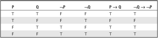
The principle of modus tollens, which we learned earlier in this chapter, depends on the law of implication reversal, also known as the law of the contrapositive:
P → Q is equivalent to ¬Q → ¬P
Table 2-22 demonstrates the law of implication reversal.
TABLE 2-21 Truth tables for the associative laws.
TABLE 2-22 Truth table for the law of implication reversal.
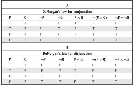
Two rules of logic show an interesting relationship among conjunction, disjunction, and negation. They’re called DeMorgan’s laws, and we can state them as follows:
• DeMorgan’s law for conjunction: ¬(P ∧ Q) ↔ ¬P ∨ ¬Q
• DeMorgan’s law for disjunction: ¬(P ∨ Q) ↔ ¬P ∧ ¬Q
TABLE 2-23 Truth tables for DeMorgan’s laws.
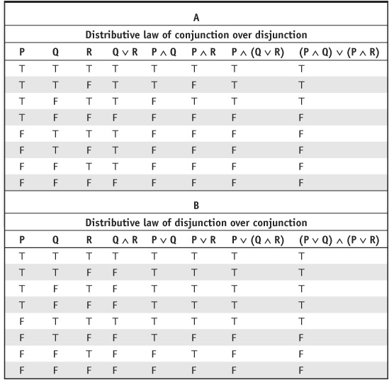
Another relationship involving conjunction and disjunction is described by the distributive laws. The first, the distributive law of conjunction over disjunction, states that a conjunction operator can be “distributed” over two disjuncts as follows:
P ∧ (Q ∨ R) ↔ (P ∧ Q) ∨ (P ∧ R)
The distributive law of disjunction over conjunction switches the roles of the two operators:
P ∨ (Q ∧ R) ↔ (P ∨ Q) ∧ (P ∨ R)
Tables 2-24A and 2-24B demonstrate these principles, which some authors refer to as the distributive properties.
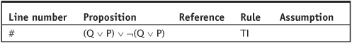
 ), Deriving Laws, and Theorem Introduction (TI)
When you have proved “both directions” of a sequent between two propositions (or sets of propositions), they are called interderivable, which implies logical equivalence. The symbol for interderivability comprises a double assertion sign, which we write as two “tee” symbols reversed and placed back to back (). Establishing interderivability requires two proofs, one for deriving the sequent “each way.”
The laws we’ve shown using truth tables can also be proved using the derivation methods described in this chapter. For example, we executed the proof for the rule of disjunction elimination for the sequent
P ∨ Q Q ∨ P
A simple substitution of propositional variables allows us to see that
Q ∨ P P ∨ Q
From the two sequents above, we can conclude the sequential expression of the commutative principle
P ∨ Q Q ∨ P
We can also prove a version of the laws as theorems within the propositional calculus. For the commutative law of disjunction, a step using the rule of conditional proof can turn the sequents above into implication statements with no assumptions, and then we can combine them into the biconditional theorem
TABLE 2-24 Truth tables for the distributive laws.
P ∨ Q ↔ Q ∨ P
When we state the above-described laws as theorems of the propositional language, we can use them in proofs by substituting in the relevant PF. For example, at any point in a proof, we can introduce the law of excluded middle and cite the rule of theorem introduction (TI), an example of which we see summarized in Table 2-25. By definition, theorems rely on no premises, so we need no references or assumptions.
TABLE 2-25 An example of theorem introduction on a line in a proof.
You can employ any of the laws you’ve seen so far, as well as any theorem you might have previously proved in the course of your logical wanderings, in a theorem introduction.
You may refer to the text in this chapter while taking this quiz. A good score is at least 8 correct. Answers are in the back of the book.
1. Which of the following portrays a correct way to read the symbol ?
I. “…therefore…”
II. “It is a theorem that…
III. “…if and only if…”
IV. “…yields…”
V. “…is a tautology.”
A. I, II, and IV are correct.
B. Only II is correct.
C. I and V are correct.
D. All of the above are correct.
2. Suppose you observe that “It is not sunny outside, and it is not hot outside.” Your friend says, “It is not the case that it is sunny or hot today.” These two sentences are logically equivalent, providing an example of
A. one of DeMorgan’s laws.
B. the law of double negation.
C. the law of implication reversal.
D. no law; the two statements are not equivalent.
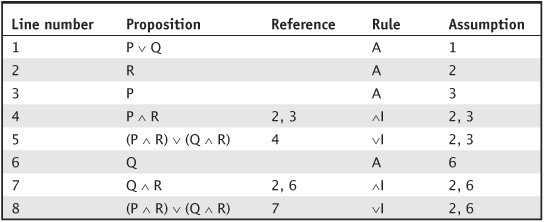
3. Which of the following statements accurately describes the proof shown in Table 2-26?
A. The table constitutes a valid proof of the sequent.
B. The proof contains errors in the assumption column, so it’s invalid.
C. The proof constitutes a valid deduction, but it does not prove the sequent.
D. The proof contains errors in the rule column, so it’s invalid.
TABLE 2-26 Proof of the sequent P ∨ Q, R (P ∧ R) ∨ (Q ∧ R).
4. What, if anything, can be done to correct the proof in Question 3?
A. The antecedent of the sequent should be changed to P ∨ Q, P ∧ R.
B. the rule at step 7 should be changed to disjunction elimination (∨E).
C. An extra step using disjunction elimination (∨E) should be added at the end.
D. Nothing needs to be done. it is correct as it is.
5. Suppose someone says to you, “If the sun is shining, it is hot outside. But it is not hot outside, so the sun must not be shining.” This is an example of
A. one of DeMorgan’s laws.
B. the distributive law of conjunction over disjunction.
C. the law of implication reversal.
D. no law; your friend’s reasoning is invalid.
6. Suppose that a mathematician says, “A number is rational if and only if it equals the ratio of two integers.” You respond by saying, “If I take an integer and divide it by another integer, I’ll end up with a rational number.” You can get this conclusion straightaway from the mathematician’s claim by invoking
A. the rule of biconditional elimination.
B. modus tollens.
C. modus ponens.
D. the law of the contrapositive.
7. If we formulate a PF, no matter how complicated, we know that it must be either true or false based on the law of
A. implication reversal.
B. contradiction.
C. excluded middle.
D. interderivability.
8. Which of the following constitute PFs according to the rigorous definition of PF construction?
I. P → (Q → R))
II. (P ∧ Q) = T
III. (P ∧ (¬P))
IV.) PQ(¬
V. ((P ∧ Q)→P)
A. I, III, and V are PFs.
B. Only III is a PF.
C. All but IV are PFs.
D. None of the above is a PF.
9. When using the rule of modus ponens (MP), we must copy over
A. the assumptions from the conditional statement and the antecedent.
B. the assumptions from the conditional statement only.
C. the assumptions from the conditional statement and the consequent.
D. nothing; modus ponens requires no assumptions.
10. If you say “It is hot and it is sunny, or it is hot and it is cloudy,” the distributive law of conjunction over disjunction allows you to conclude
A. nothing, because the law does not properly apply to this statement.
B. the equivalent statement “It is not cloudy and it is sunny, or it is cloudy and not sunny.”
C. the equivalent statement “If it is cloudy or sunny, then it is hot.”
D. the equivalent statement “It is hot outside, and sunny or cloudy.”