CHAPTER 5
Error Maximization
FALLACY: OPTIMIZED PORTFOLIOS ARE HYPERSENSITIVE TO INPUT ERRORS
Mean‐variance analysis requires investors to estimate expected returns, standard deviations, and correlations whose future realizations will vary from their estimated values. The process of optimization, by construction, will overallocate to asset classes for which expected returns are overestimated and for which standard deviations and correlations are underestimated, and it will underallocate to asset classes for which the opposite occurs. Moreover, the effect of estimation error is not diversified away as more asset classes are added; it usually becomes worse.
The effect of this problem is twofold: The weights of the efficient portfolios are misstated, and their expected returns and risk are incorrect. The question arises, therefore, as to the seriousness of this problem. Are optimizers so sensitive to errors as to be of little or no value, or are critics of optimization overstating this problem? We believe the latter is true. In most cases, and in particular, for applications to asset allocation, optimization is reasonably robust to estimation error.
THE INTUITIVE ARGUMENT
The intuition of our argument is straightforward. Consider optimization among asset classes that have similar expected returns and risk. Small errors in the estimates of these values may substantially misstate efficient allocations. Despite these misallocations, however, the return distributions of the correct and incorrect portfolios will be quite similar. In this setting we assume that portfolio weights are constrained to disallow leverage, which is typically the case. And even if we assume reasonable amounts of leverage, our result would typically still hold.
Now consider optimization among asset classes that have dissimilar expected returns and risk. Small errors in these estimates will have little impact on efficient allocations; hence, again the return distributions of the correct and incorrect portfolios will not differ much. The following examples illustrate these points.
THE EMPIRICAL ARGUMENT
Country Allocation
Let's first consider an application of mean‐variance analysis to the developed equity markets of France, Germany, and the United Kingdom. Table 5.1 shows estimates of expected returns, standard deviations, and correlations. The expected returns are those that would occur if these assets were fairly valued given their historical covariances with the world equity market measured over the period from January 1976 through December 2015, which is to say that these returns are proportional to their historical betas. The standard deviations and correlations are calculated from the same historical sample.
TABLE 5.1 Country Expected Returns, Standard Deviations, and Correlations
| Correlations | ||||
| Expected Returns | Standard Deviations | France | Germany | |
| France | 7.8% | 25.3% | ||
| Germany | 7.6% | 25.0% | 0.75 | |
| United Kingdom | 7.3% | 21.5% | 0.66 | 0.60 |
Notice that these asset classes are close substitutes for each other given these assumptions about return and risk. The spread between the highest and lowest expected return is only 50 basis points, and there is little dispersion across the standard deviations and correlations.
Now suppose we wish to identify the optimal mix of these country equity markets, but we misestimate the expected returns. Specifically, we overestimate the expected returns of France and the United Kingdom by 1.00 percent, and we underestimate the expected return of Germany by 1.00 percent. We assume that we estimate the standard deviations and correlations correctly. Table 5.2 shows these misestimated expected returns.
TABLE 5.2 Misestimated Country Expected Returns
| Correct Expected Returns | Errors | Expected Returns with Errors | |
| France | 7.8% | +1% | 8.8% |
| Germany | 7.6% | −1% | 6.6% |
| United Kingdom | 7.3% | +1% | 8.3% |
Table 5.3 shows that these errors significantly distort the optimal portfolio when we apply mean‐variance analysis.1 The optimization process overweights asset classes for which we have overestimated expected returns and it underweights the asset class for which we have underestimated expected return. In total, more than 62 percent of the portfolio is misallocated.
TABLE 5.3 Distortion in Optimal Country Weights
| Correct Weights | Incorrect Weights | Misallocation | |
| France | 25.5% | −5.7% | −31.2% |
| Germany | 23.8% | 44.9% | 21.1% |
| United Kingdom | 50.7% | 60.8% | 10.1% |
| Total Misallocation | 62.4% |
This example shows that small errors in our estimates of expected returns substantially distort a portfolio's optimal weights, suggesting that optimizers are indeed hypersensitive to input errors. But is such a conclusion warranted? Although the portfolio resulting from the misestimated means is substantially misallocated, the return distribution of the perceived optimal portfolio is similar to the return distribution of the true optimal portfolio. Table 5.4, which shows each portfolio's exposure to loss, illustrates this point.
TABLE 5.4 Exposure to Loss for Correct and Incorrect Country Weights
| Correct Weights | Incorrect Weights | |
| Probability of Loss | 16.1% | 16.7% |
| 1% Value at Risk | −58.4% | −59.2% |
The misallocated portfolio has a 16.7 percent likelihood of experiencing a loss over a one‐year horizon, whereas the truly optimal portfolio has a 16.1 percent chance of losing money during a single year. In other words, a massive 60 percent misallocation translates into a mere 0.6 percent increase in exposure to loss.
The same is true if we consider exposure to loss as value at risk, which gives the worst outcome for a given probability. Over a one‐year horizon, the worst outcome for the truly optimal portfolio given a 1 percent probability of occurrence is a loss of 58.4 percent, which increases to only 59.2 percent if we misallocate the portfolio by more than 60 percent.
The bottom line is that if asset classes have similar return distributions, small errors in their estimated means will lead to large errors in the composition of the perceived optimal portfolio. This sensitivity of the weights to errors in the means occurs because the assets are close substitutes for one another. But because they are close substitutes, the misallocations have comparatively little impact on the portfolio's return distribution. In other words, although a portfolio's weights may be hypersensitive to input errors, the risk profile of the incorrect portfolio is very similar to the risk profile of the truly optimal portfolio.
Asset Allocation
Now let us explore a situation in which the asset classes are less similar to each other. Table 5.5 shows expected returns, standard deviations, and correlations for three asset classes: U.S. equities, Treasury bonds, and commodities. The standard deviations and correlations are estimated from monthly returns beginning in January 1976 and ending in December 2015. The expected returns are the same returns we used for our base case example in Chapter 2. For the sake of this experiment, we assume these inputs are the true values that will prevail in the future.
TABLE 5.5 Asset Class Expected Returns, Standard Deviations, and Correlations
| Correlations | ||||
| Expected Returns | Standard Deviations | U.S. Equities | Treasury Bonds | |
| U.S. Equities | 8.8% | 16.6% | ||
| Treasury Bonds | 4.1% | 5.7% | 0.10 | |
| Commodities | 6.2% | 20.6% | 0.16 | −0.07 |
Notice that the spread in expected returns is 4.7 percent compared to 50 basis points for the country allocation example. Moreover, the standard deviations and correlations are quite dissimilar compared to those of the country equity indexes.
Again, suppose we wish to allocate our portfolio optimally across these asset classes, but we overestimate the expected returns of U.S. equities and commodities by 1.00 percent and underestimate the expected return of Treasury bonds by 1.00 percent.2 Table 5.6 shows these incorrect assumptions.
TABLE 5.6 Misestimated Asset Class Expected Returns
| Correct Expected Returns | Errors | Expected Returns with Errors | |
| U.S. Equities | 8.8% | +1% | 9.8% |
| Treasury Bonds | 4.1% | −1% | 3.1% |
| Commodities | 6.2% | +1% | 7.2% |
Table 5.7 reveals that, unlike the previous example, small errors in the estimates of expected returns result in relatively small misallocations. We would incur only 23.5 percent turnover in order to shift the portfolio from the incorrect weights to the correct weights compared to nearly three times as much for countries.
TABLE 5.7 Distortion in Optimal Asset Class Weights
| Correct Weights | Incorrect Weights | Misallocation | |
| U.S. Equities | 66.7% | 55.0% | −11.7% |
| Treasury Bonds | 19.8% | 27.0% | 7.2% |
| Commodities | 13.5% | 18.0% | 4.5% |
| Total Misallocation | 23.5% |
Table 5.8 compares exposure to loss for the truly optimal asset class portfolio with exposure to loss for the misallocated asset class portfolio. It reveals that the differences again are relatively minor, but this time because the misallocation is within reason.
TABLE 5.8 Exposure to Loss for Correct and Incorrect Asset Class Weights
| Correct Weights | Incorrect Weights | |
| Probability of Loss | 1.9% | 1.3% |
| 1% Value at Risk | −9.5% | −3.6% |
THE ANALYTICAL ARGUMENT
We now address the sensitivity of optimized portfolios to changes in expected return using explicit mathematical formulas. Specifically, we compute the partial derivative (rate of change) of optimal weights with respect to a change in any of the asset classes' expected returns. We also compute the partial derivative of the optimal portfolio's standard deviation with respect to these changes in expected returns.
We start by expressing the optimal weights as a function of means, covariances, and risk aversion, for an unconstrained portfolio. These optimal weights are given by the following formula, where  is a risk aversion parameter,
  is the covariance matrix, and
  is a vector of expected returns:
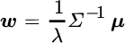
However, this optimization setup is problematic in a practical context. This formula implies that investors will increase exposure to asset classes with higher expected returns and thereby increase total risk, even employing leverage if necessary. In practice, the opposite reaction is more likely. Though investors will allocate too much to asset classes whose expected returns have been erroneously inflated, they will have an overly optimistic view of expected return and, if they target a particular return or risk level, they will substitute safer and therefore lower‐return asset classes elsewhere in their portfolio. This behavior is consistent with two simple constraints: portfolio weights sum to 1, and the investor targets a specific expected return. Fortunately, it is possible to derive a formula for these optimal weights in terms of the expected returns, covariances, and a target expected return,  :
:

Interestingly, this solution is based on a weighted average of two portfolios:  , which is proportional to the unconstrained solution we described previously, and
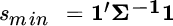
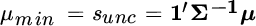
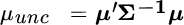
  , which is proportional to the minimum‐variance portfolio (because when all expected returns are equal to the same positive constant, optimization equates to risk minimization). The coefficients that blend these two portfolios are based on the means and the sum of weights associated with the two portfolios, and the weights are normalized by a factor we call
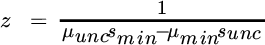
  . These quantities are defined as follows:
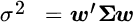
The optimal portfolio's variance is equal to:

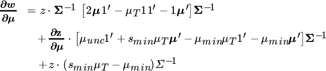
Using standard calculus and matrix algebra rules, we take the partial derivative of the weights with respect to changes in expected returns. Because the weights are a vector, the partial derivative of it with respect to another vector (expected returns) produces a matrix in which each column describes the amount each weight changes given a one‐unit change in each of the expected returns. The expression below is long, but we will soon be able to compare it directly to the derivative of standard deviation.
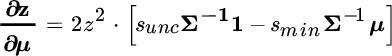
For reasons that will become clear soon, we leave  expressed as such in the derivative, but note that it is equal to:
We express the derivative of portfolio variance with respect to changes in expected returns in a similar fashion. In this case, variance is a single number, so its derivative is a column vector of sensitivities to changes in each expected return.
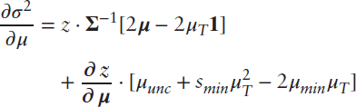
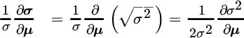
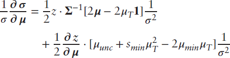
The derivative of weights is in intuitive units, because changes in weights occur against a backdrop of a set of weights that sum to 1. For variance, though, it is hard to say whether a particular change is large or small when the size of the variance itself differs across portfolios. We make two adjustments to this equation for variance in order to facilitate our interpretation of risk sensitivity. First, we recast the derivative in terms of standard deviation, which is the square root of variance. And second, we divide by the standard deviation of the original portfolio to put the size of each change in context. After these two changes, we have the following relationships:
As with any derivative, these sensitivities are linear approximations, which hold quite closely for small changes in expected returns but are less accurate for larger changes. We confirm the level of accuracy by introducing small perturbations in expected returns and by recomputing portfolio weights from Equation (5.2), which are predicted by the derivatives in Equations (5.9) and (5.13). It is precisely the small changes we are concerned with in evaluating stability, so we are able to derive a good amount of intuition from these relationships.
A visual comparison of Equations (5.9) and (5.13) suggests that weight sensitivity and standard deviation sensitivity have some similarities. The first term (on the first line) in each formula involves  ,
,  , and a similar expression inside the brackets. Whereas the weight formula is multiplied by the inverse covariance matrix at the end, the standard deviation formula is multiplied by
  , which is the inverse variance of the entire portfolio. Importantly, the term in the standard deviation formula is divided by 2 compared to the weight formula. This suggests that, on average, this component of standard deviation is less sensitive than the analogous component of optimal weights. The next terms (on the second lines of the formulas) are also similar. They both involve
  and a related expression inside the brackets. Once again, they are multiplied at the end by the inverse covariance matrix and inverse portfolio variance, respectively, and the standard deviation formula is divided by 2. The weight formula also has a third expression, for which the standard deviation formula has no parallel. It is, in fact, this component that leads to most of the instability in weights. It is a scalar multiple of the inverse covariance matrix, and the inverse covariance matrix is the quantity that “blows up” when assets are highly correlated. (Think of the covariance matrix as describing risk, and the inverse covariance matrix as describing how to neutralize this risk. When two assets are highly correlated, we neutralize their risk by taking massive long positions in one and massive short positions in the other.)
To quantify these differences, we apply these formulas to our portfolio example from Chapter 2. We ignore cash equivalents because their risk is close to zero; instead, we focus on the remaining six asset classes. We set the target return equal to 7.5 percent. The moderate portfolio does not hold any cash equivalents, so with these assumptions, Equation (5.2) yields exactly the same moderate portfolio as we have shown previously. Table 5.9 shows the sensitivity of each optimal weight (in the columns) to a one percentage point increase in the expected return of each asset individually (in the rows). For example, the expected return of U.S. equities increases from 8.8 percent to 9.8 percent. Table 5.10 shows the sensitivity of the optimal portfolio's standard deviation. We observe the following. Weights are not very sensitive to expected return errors in an asset class such as commodities, which is relatively dissimilar from other asset classes. And because the weights do not change by much, neither does the portfolio's standard deviation. On the other hand, when the change in expected return is applied to an asset class such as Treasury bonds, which is a close substitute for U.S. corporate bonds, the weights change by around 200 percent. This is of little consequence, though; the assets are indeed close substitutes with similar risk properties; hence, the risk of the total portfolio remains stable.
TABLE 5.9 Sensitivity of Weights to Changes in Expected Return
| Weight Sensitivity | ||||||
| U.S. Equities | Foreign Equities | Emerging Market Equities | Treasury Bonds | U.S. Corporate Bonds | Commodities | |
| Sensitivity of Weights to 1% Increase in Expected Return | ||||||
| U.S. Equities | 19% | −11% | −6% | 18% | −21% | 1% |
| Foreign Developed Market Equities | −11% | 17% | −7% | 16% | −13% | −2% |
| Emerging Market Equities | −6% | −7% | 9% | 17% | −13% | −1% |
| Treasury Bonds | 7% | 6% | 14% | 191% | −212% | −7% |
| U.S. Corporate Bonds | −17% | −9% | −12% | −200% | 235% | 2% |
| Commodities | 0% | −3% | −1% | −5% | 1% | 7% |
TABLE 5.10 Sensitivity of Portfolio Standard Deviation to Changes in Expected Return
| Original Standard Deviation | New Standard Deviation | Percentage Change in Risk | ||
| Sensitivity of Standard Deviation to 1% Increase in Expected Return | ||||
| U.S. Equities | 10.8% | 10.1% | −6.5% | |
| Foreign Developed Market Equities | 10.8% | 10.2% | −5.9% | |
| Emerging Market Equities | 10.8% | 10.6% | −2.3% | |
| Treasury Bonds | 10.8% | 10.4% | −3.6% | |
| U.S. Corporate Bonds | 10.8% | 10.2% | −5.6% | |
| Commodities | 10.8% | 10.7% | −1.5% | |
THE BOTTOM LINE
The bottom line is that mean‐variance analysis is not typically hypersensitive to estimation error. It only appears to be hypersensitive when asset classes are close substitutes for each other, because the optimal weights may shift significantly in response to input errors. But the incorrect portfolio will have a similar return distribution as the correct portfolio; thus, variation in weights may not be overly problematic.
Nonetheless, there are some situations in which estimation error poses a significant challenge to investors. Fortunately, we have procedures to address this challenge. Some investors resort to Bayesian shrinkage, which blends individual estimates of expected return and risk with a prior belief such as the cross‐sectional mean of the estimates or the estimate associated with the minimum‐risk portfolio. Investors also rely on a technique called resampling in which they generate many efficient frontiers from a distribution of inputs and then average the weights of the portfolios with a given risk level to arrive at the optimal portfolio.3 Both of these techniques are designed to make a portfolio less sensitive to estimation error. An alternative approach, called stability‐adjusted optimization, addresses estimation error in a much different way. It makes portfolios more sensitive to estimation error, but in a constructive way. This approach measures the relative stability of covariances and incorporates this information as a distinct component of risk in the portfolio formation process. It increases dependency on asset classes with relatively stable covariances and reduces dependency on asset classes with relatively unstable covariances. In Chapter 13 we discuss stability‐adjusted optimization in detail.
REFERENCES
- R. O. Michaud and R. O. Michaud. 2008. Efficient Asset Management: A Practical Guide to Stock Portfolio Optimization and Asset Allocation, Second Edition (New York: Oxford University Press, Inc.).