CHAPTER 9
Constraints
THE CHALLENGE
Investors who deploy optimization to form portfolios often intervene in the optimization process by constraining allocation to certain asset classes. Constraints, however, reduce a portfolio's efficiency. We show how to produce more efficient portfolios without imposing constraints. And at the same time, we address the concerns that induce investors to impose constraints in the first place.
WRONG AND ALONE
Why do investors constrain their portfolios knowing that these constraints will produce a suboptimal result, given their views about expected return and risk? The argument typically put forth is that investors lack sufficient conviction in their views. We disagree. Consider the following thought experiment. Imagine you know for certain the long‐term future means, standard deviations, and correlations of the asset classes that you use to form your portfolio. Your conviction is, therefore, absolute. Nonetheless, it is likely that you will still be reluctant to allocate your portfolio in such a way that is notably different from the norm, because within short subperiods the asset class returns most likely will diverge substantially from their long‐term means, both positively and negatively, merely as a function of their standard deviations. You may well be able to tolerate subperiods of poor performance if most other investors experience similar poor performance, but you would likely be much less comfortable if you were the only investor to experience poor performance. Investors take comfort in the company of others when they perform poorly. We argue that investors constrain their portfolios, not because they lack conviction in their views but, rather, because they are averse to being wrong and alone—wrong because they perform poorly during a particular subperiod, and alone because they are the only one to perform poorly at that time. Table 9.1 illustrates the potential outcomes when investors care simultaneously about absolute and relative performance.
TABLE 9.1 Potential Absolute and Relative Performance Outcomes
| Absolute Returns | ||
| Relative Returns | Favorable | Unfavorable |
| Favorable | 1. Great | 2. Tolerable |
| Unfavorable | 3. Tolerable | 4. Very Unpleasant |
If we accept that investors care not only about how they perform in an absolute sense but also about how their performance compares to that of other investors, there are four possible outcomes. An investor could achieve favorable absolute returns and at the same time outperform his or her peers, which would be great, as represented by Quadrant 1. Alternatively, an investor might outperform the competition but fall short of an absolute target (Quadrant 2). Or an investor might generate a high absolute return but underperform the competition (Quadrant 3). Quadrants 2 and 3 would probably be tolerable because the investor would produce superior performance along at least one dimension. However, it would likely be very unpleasant if an investor generated an unfavorable absolute result and at the same time performed poorly relative to other investors (Quadrant 4). It is the fear of this outcome that induces investors to constrain their portfolios toward a “normal” asset mix.
MEAN‐VARIANCE‐TRACKING ERROR OPTIMIZATION
Although the imposition of constraints reduces the odds of being wrong and alone, it does so inefficiently because investors choose constraints arbitrarily.
Recall from Chapter 2 that we identify portfolios along the efficient frontier by maximizing expected utility as shown in Equation (9.1).
In Equation (9.1),  equals expected utility,
  equals portfolio expected return, and
  equals risk aversion, and
  equals portfolio standard deviation.
When investors impose constraints on the optimization process, they are employing an ad hoc procedure for addressing their aversion to tracking error (being alone). Tracking error is a measure of relative risk. Just as standard deviation measures dispersion around an average return, tracking error also measures dispersion, but instead around the average relative return between a portfolio and its benchmark. Imagine subtracting a sequence of benchmark returns from a sequence of portfolio returns covering the same period. The standard deviation of these differences is what we call tracking error.
If we care only about relative performance, we could define our returns net of a benchmark and optimize in dimensions of expected relative return and tracking error. This approach would address our concern about deviating from the norm, assuming our benchmark represents normal investment choices. However, we would fail to address any concern we might have about absolute results. Given that investors likely care about both absolute and relative performance, we should expand expected utility to encompass both dimensions of risk, as shown in Equation (9.2).1

Here,  equals tracking error aversion, and
  equals portfolio tracking error. We can express this multirisk expected utility formula as a function of the portfolio weight vector, noting that tracking error is the standard deviation of relative returns against the benchmark portfolio,
  :
:

Notice that the objective function does not include a term for expected relative return. There is no need to distinguish between expected absolute return and expected relative return because they differ only by the expected return of the benchmark, which is a constant value independent of the portfolio weights. By maximizing expected absolute return we are effectively maximizing expected relative return. However, standard deviation and tracking error are not linearly related; thus, we must include both risk terms.
Efficient Surface
This measure of investor satisfaction simultaneously addresses concerns about absolute and relative performance. Instead of producing an efficient frontier in two dimensions, though, this optimization process produces an efficient surface in three dimensions: expected return, standard deviation, and tracking error, as displayed in Figure 9.1.

FIGURE 9.1 Efficient Surface
The efficient surface is bounded on the upper left by the traditional mean‐variance (MV) efficient frontier, which includes efficient portfolios in dimensions of expected return and standard deviation. The right boundary of the efficient surface is the mean‐tracking error (MTE) efficient frontier. It comprises portfolios that offer the highest expected return for varying levels of tracking error. The efficient surface is bounded on the bottom by combinations of the least risky portfolio and the benchmark portfolio. The lower left corner of the efficient surface is the least risky portfolio in terms of standard deviation. The upper right corner of the efficient surface is a portfolio that is allocated entirely to the asset class with the highest expected return. The lower right corner of the efficient surface is the benchmark portfolio, which has no tracking error.
All of the portfolios that lie on this surface are efficient in three dimensions. It does not follow, however, that a three‐dimensional efficient portfolio is efficient in any two dimensions. Only the maximum expected return portfolio is efficient in all three dimensions. Consider, for example, the least risky portfolio. Although it is on both the mean‐variance efficient frontier and the efficient surface, if it were plotted in dimensions of just expected return and tracking error, it would appear very inefficient compared to a benchmark that includes high‐expected‐return assets such as stocks and long‐term bonds. This portfolio has a low expected return compared to the benchmark and yet a high degree of tracking error.
We should expect this approach to optimization to deliver results that are superior to constrained mean‐variance optimization in the following sense. For a given combination of expected return and standard deviation, it should produce a portfolio with less tracking error. Or for a given combination of expected return and tracking error, it should identify a portfolio with a lower standard deviation. Or, finally, for a given combination of standard deviation and tracking error, it should deliver a portfolio with a higher expected return than constrained mean‐variance analysis. Most of the portfolios identified by constrained mean‐variance analysis would lie beneath the efficient surface. In fact, the only way in which mean‐variance‐tracking error optimization would fail to improve upon a constrained mean‐variance analysis is if the investor knew in advance what constraints were optimal. But, of course, this knowledge could only come from a mean‐variance‐tracking error optimization.
Iso‐Expected Return Curve
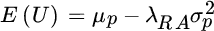
Some investors may be more concerned about absolute performance, while others may care more about relative performance. We can construct an iso‐expected return curve to assist investors in addressing this trade‐off. An iso‐expected return curve plots portfolios that all have the same expected return in dimensions of standard deviation and tracking error, as shown in Figure 9.2.
FIGURE 9.2 Iso‐Expected Return Curve
Investors who worry more about absolute performance will prefer portfolios to the left on the iso‐expected return curve, while those who are more concerned with tracking error will prefer portfolios further to the right on the curve. There is a unique iso‐expected return curve for every level of expected return.
The bottom line is that constrained mean‐variance optimization is inefficient because it arbitrarily determines the maximum or minimum allocation to various asset classes. Investors resort to constraints because they are fearful of performing poorly while deviating from the norm. Investors can address this issue more efficiently by identifying a benchmark that represents a “normal asset allocation” and expanding their objective function to include terms for aversion to tracking error.
REFERENCES
- G. Chow. 1995. “Portfolio Selection Based on Return, Risk, and Relative Performance,” Financial Analysts Journal, Vol. 51, No. 2 (March/April).