CHAPTER 14
Leverage versus Concentration

THE CHALLENGE

Theory shows that it is preferable to apply leverage to a less risky portfolio than to concentrate a portfolio in riskier assets for the purpose of raising expected return. This theoretical result, however, relies upon assumptions that may be only partially valid, if at all. In this chapter, we relax the assumptions that produce this theoretical result to match real‐world conditions, and we reexamine the efficacy of leverage and concentration. We find that what is inarguable theoretically does not always hold empirically when we introduce more plausible assumptions.

LEVERAGE IN THEORY

The notion that investors are better served by applying leverage to a less risky portfolio rather than concentrating a portfolio in riskier assets in order to raise expected return has an impressive theoretical lineage. As we discussed in Chapter 2, Markowitz (1952) introduced portfolio theory, which shows how to combine risky assets into efficient portfolios that yield the highest expected return for a given level of risk. He called a continuum of such portfolios the efficient frontier. Tobin (1958) showed that the investment process can be separated into two distinct steps: the construction of an efficient portfolio as described by Markowitz, and the decision to combine this efficient portfolio with a risk‐free investment. This two‐step process is called the separation theorem. Tobin showed that there is a unique portfolio along the efficient frontier, which, when combined with lending or borrowing at the risk‐free interest rate, dominates all other portfolios along the efficient frontier. This is the tangency portfolio denoted as M in Figure 14.1. The curved line represents the efficient frontier, while the straight line emanating from the vertical axis at the risk‐free rate depicts the efficient frontier with borrowing or lending. It is called the capital market line. The segment of the capital market line between the vertical axis and its tangency point with the efficient frontier represents a combination of lending and portfolio M. That segment of the capital market line that continues beyond portfolio M represents a combination of portfolio M and borrowing at the risk‐free rate, which is to say, leverage.

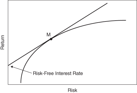
FIGURE 14.1 Efficient Frontier with Borrowing and Lending

Sharpe (1964) extended Markowitz's and Tobin's insights to develop a theory of market equilibrium under conditions of risk, which he called the Capital Asset Pricing Model. Sharpe showed that portfolio M is the market portfolio comprising all investable assets in proportion to their total value, assuming all investors have identical expectations for returns, standard deviations, and correlations. In equilibrium, the market portfolio offers the maximum achievable diversification. It follows that investors who seek returns above or below the expected return of the market portfolio prefer points along the capital market line as opposed to the efficient frontier, because these combinations of the market portfolio and borrowing or lending offer less risk than portfolios along the efficient frontier. Or, for investors who target a given level of risk, it follows that leveraging lower‐risk asset classes increases expected returns more than concentrating a portfolio in riskier asset classes.

Each building block of this elegant result rests on certain assumptions, which may be convenient but often fail to conform to real‐world conditions. Portfolio theory, for example, assumes either that returns are elliptically distributed or that investor preferences are well approximated by mean and variance. It also assumes implicitly that investors can estimate expected returns, standard deviations, and correlations reasonably well. The separation theorem assumes that investors can borrow or lend an unlimited amount of funds at the risk‐free rate without being required to meet margin calls or to post collateral. And the Capital Asset Pricing Model assumes that investors have the same expectations for returns, standard deviations, and correlations. We relax these assumptions individually, and then collectively, to accord with real‐world conditions.

We first assume that investor preferences may be better described by a kinked utility function than a smooth concave function, and we combine this assumption with empirical distributions that are not elliptically distributed.

Next, we acknowledge that investors make errors when they estimate expected returns, standard deviations, and correlations. We consider three types of estimation error: independent‐sample error, interval error, and small‐sample error. Independent‐sample error refers to the discrepancy between historical mean returns, standard deviations, and correlations and future realizations of these values. Interval error refers to the discrepancy between standard deviations and correlations estimated from high‐frequency observations, such as monthly returns, and longer‐horizon extrapolations of these values, such as annual and multiyear standard deviations and correlations. To the extent lagged correlations are nonzero, standard deviations do not scale with the square root of time, and correlations differ depending on the return interval used to estimate them. Small‐sample error addresses the fact that investors typically use large samples of historical returns to determine the expected returns, standard deviations, and correlations of smaller samples. (See Chapter 13 for more detail about estimation error.)

Next, we relax the assumption that investors can borrow at the risk‐free rate by adding a premium to this rate. We could extend this analysis to account for collateral, margin calls, and the opportunity cost of deploying capital to collateralize borrowing instead of deploying it in more productive ways. For simplicity, we do not account for these complexities in this chapter.

Finally, we allow for heterogeneous expectations of returns, standard deviations, and correlations by assuming certain investors are skilled at forecasting future returns.

LEVERAGE IN PRACTICE

The aggressive portfolio we derived in Chapter 2 has an expected return of 9 percent. Suppose this return is not sufficient for our needs. What if we require a 10 percent expected return? One way to achieve this outcome is to concentrate the portfolio in asset classes with higher expected returns. This optimal portfolio, which is close to the right end of the efficient frontier, is shown in the first column of Table 14.1. Another way to increase expected return is to lever the portfolio. The second column of Table 14.1 shows the optimal levered portfolio that has the same risk as the concentrated portfolio. The expected return of the levered portfolio minus the expected return of the concentrated portfolio equals 0.37 percent. Given our assumptions, we would expect the levered portfolio to outperform the concentrated portfolio by 0.37 percent per year.

TABLE 14.1 Leverage versus Concentration in Theory

	Optimal Concentrated Portfolio Weights (%)	Optimal Levered Portfolio Weights (%)
U.S. Equities	25.2%	43.7%
Foreign Developed Market Equities	39.2%	39.7%
Emerging Market Equities	35.6%	15.6%
Treasury Bonds	0.0%	39.2%
U.S. Corporate Bonds	0.0%	31.5%
Commodities	0.0%	10.7%
Borrowing	0.0%	–80.4%
Sum of Weights	100.0%	100.0%
Expected Return	10.0%	10.4%
Standard Deviation	18.6%	18.6%
Sharpe Ratio	0.35	0.37
Excess Return of Levered Portfolio		0.37%

Because we have employed mean‐variance analysis to identify these portfolios, the results presume that asset class returns are elliptically distributed or that investor preferences are well approximated by mean and variance. Neither assumption is literally true. We relax these assumptions in two distinct ways. First, we estimate the semi–standard deviation of the concentrated and levered portfolios from Table 14.1 given a nonelliptical distribution. The semi–standard deviation is simply the standard deviation calculated using the subsample of returns for each asset class that fall below the full‐sample mean.¹ We also calculate the Sortino ratio, which is equivalent to the Sharpe ratio but with semi–standard deviation as the denominator. Second, we calculate the expected utility of each portfolio based on a kinked utility function and convert these expected utilities into their certainty equivalent values.² These results are shown in Table 14.2.

TABLE 14.2 Leverage versus Concentration with Nonelliptical Returns and Kinked Utility

	Optimal Concentrated Portfolio	Optimal Levered Portfolio
Expected Return	10.0%	10.4%
Standard Deviation	18.6%	18.6%
Sharpe Ratio	0.35%	0.37%
Semi–Standard Deviation	19.5%	0.36%
Sortino Ratio	0.33%	35.5%
Implied Return at 18.6% Semi–Standard Deviation	9.7%	10.1%
Excess Return of Levered Portfolio		0.42%
Kinked Utility (levered − concentrated)*		2.4%
Certainty Equivalent (levered − concentrated)		0.38%

*This table shows average utility of each portfolio over our sample period. We derive kinked utility assuming a kink at –5%, curvature of 5, and annual periodicity.

While the levered and concentrated portfolios have the same standard deviation by design, they have different semi–standard deviations. Therefore, to make the returns comparable, we must adjust them based on their semi–standard deviation. To do this, we simply multiply the Sortino ratio of each portfolio by the standard deviation of 18.6 percent and add the risk‐free rate of 3.5 percent. This calculation tells us the return we should expect from each portfolio, assuming they have the same semi–standard deviation. Interestingly, the levered portfolio outperforms the concentrated portfolio by 0.42 percent. When we lift these assumptions, we find that the levered portfolio is expected to outperform the concentrated portfolio by an even greater margin. This result is counterintuitive in the sense that most investors might expect leverage to amplify, rather than reduce, the impact of nonnormal distributions and asymmetric preferences. A closer inspection of the asset class semivariances provides insight into this result.

Table 14.3 reveals that equities and commodities have semi–standard deviations that exceed their standard deviations, whereas fixed‐income asset classes have semi–standard deviations that are lower than their standard deviations. Because the levered portfolio is allocated 60 percent to fixed income, whereas the concentrated portfolio is allocated entirely to equities, the former has a lower semi–standard deviation than the latter. In this specific example, the normality assumption actually leads us to underestimate the outperformance of leverage relative to concentration.

TABLE 14.3 Asset Class Semi–Standard Deviations

	Semi–Standard Deviation (%)	Standard Deviation (%)	Semi minus Full (%)
U.S. Equities	17.4	16.6	0.9
Foreign Developed Market Equities	19.5	18.6	0.9
Emerging Market Equities	28.0	26.6	1.4
Treasury Bonds	5.3	5.7	–0.4
U.S. Corporate Bonds	7.0	7.3	–0.3
Commodities	21.4	20.6	0.8
Cash Equivalents	1.0	1.1	–0.1

The bottom two rows of Table 14.2 compare the levered and concentrated portfolios through the lens of a kinked utility function. We see from these results that the levered portfolio offers higher kinked utility than the concentrated portfolio, which is consistent with our analysis of semi–standard deviation. While both portfolios experience returns below the kink approximately 20 percent of the time, the average loss below the kink is larger for the concentrated portfolio. We convert these average expected utilities into certainty equivalents by reversing the expected utility function (which expresses expected utility in terms of return) to solve for the return as a function of expected utility. We find that the levered portfolio has a certainty equivalent that is 0.38 percent higher than the concentrated portfolio.

Next, we lift the assumption that investors can estimate returns and covariances reliably and that standard deviation scales with the square root of time. We do this in the same manner as we did in Chapter 13.

1. We partition our returns data into a testing subsample (the first 60 months in the sample) and a training subsample (the remaining 420 months in the sample).
2. We estimate the asset class covariances from the training subsample by annualizing monthly values.
3. We construct a concentrated portfolio with an expected return of 10 percent. For the expected return of each asset class, we use the full‐sample expected returns from Chapter 2. This introduces estimation error because the returns realized in each testing subsample differ, often significantly, from the full‐sample values. For the expected covariance matrix, we use the annualized covariance matrix from the training subsample.
4. We construct a levered portfolio with the same expected standard deviation as the concentrated portfolio, based on the same return and covariance assumptions.
5. We record the realized return and standard deviation of the concentrated and levered portfolios based on the outcomes in the testing subsample. We use rolling one‐year returns from the testing subsample to estimate covariances.
6. We roll the testing subsample forward one year, and repeat these steps until we have results for 36 testing samples. For each iteration, the training subsample includes all months in the full sample that are before and after the testing sample.

The results from this experiment, which we show in Table 14.4, account for independent‐sample error, interval error, and small‐sample error. In this table, the realized returns, standard deviations, and Sharpe ratios are averages across the 36 training subsamples. Because we average each measure individually, the reported return, standard deviation, and Sharpe ratio are not internally consistent. Therefore, to compare the levered and concentrated portfolios on a risk‐equivalent basis, we multiply their average Sharpe ratios by their standard deviation of 18.6 percent. We find that leverage underperforms concentration by 47 basis points in the presence of estimation error. The likely cause of this underperformance is the tendency of the levered portfolio to magnify errors because it is less constrained than the concentrated portfolio.

TABLE 14.4 Leverage versus Concentration with Estimation Error

	Optimal Concentrated Portfolio	Optimal Levered Portfolio
Average Realized Return	11.3%	11.4%
Average Realized Standard Deviation	16.8%	18.2%
Average Sharpe Ratio	0.54%	0.51%
Implied Return at 18.6% Standard Deviation	13.5%	13.0%
Excess Return of Levered Portfolio		–0.47%

Next, we return to our theoretical baseline and relax the assumption that the investor can borrow at the risk‐free rate. Specifically, we increase the borrowing cost by 25 basis points per year, such that the investor borrows at a rate of 3.75 percent (0.25 plus the risk‐free rate of 3.5 percent).

Table 14.5 reveals that borrowing costs reduce the outperformance of the levered portfolio from 37 basis points to 17 basis points. A more comprehensive analysis could incorporate the opportunity costs associated with collateral and margin requirements; however, we do not account for those complexities here.

TABLE 14.5 Leverage versus Concentration with Borrowing Costs

	Optimal Concentrated Portfolio	Optimal Levered Portfolio
Expected Return	10.0%	10.2%
Standard Deviation	18.6%	18.6%
Sharpe Ratio	0.35	0.36
Excess Return of Levered Portfolio		0.17%

Next, we lift all of the previously mentioned assumptions at the same time. These results are shown in Table 14.6. When we account for the real‐world complexities of kinked utility with nonelliptical distributions, estimation error, and higher borrowing costs, we find that the levered portfolio underperforms the concentrated portfolio by 0.83 percent on a risk‐equivalent basis.

TABLE 14.6 Leverage versus Concentration with Kinked Utility, Nonellipticality, Estimation Error, and Higher Borrowing Costs

	Optimal Concentrated Portfolio	Optimal Levered Portfolio
Average Realized Return	11.3%	11.1%
Average Realized Standard Deviation	17.2%	18.8%
Average Sortino Ratio	0.56	0.52
Implied Return at 18.6% Standard Deviation	10.5%	9.6%
Excess Return of Levered Portfolio		–0.83%

The final assumption that we relax is that investors have homogeneous expectations for returns, standard deviations, and correlations. To introduce forecasting skill to our simulations, we modify the expected returns in each of the optimizations to incorporate information from the testing sample. Specifically, we compute a weighted average expected return with a 95 percent weight on the full‐sample expected returns from Chapter 2 and a 5 percent weight on the period‐specific average returns from the testing samples. Effectively, 5 percent of the expected returns is in sample. Even a small amount of information about future outcomes has a dramatic impact on performance. Figure 14.2 summarizes the impact of lifting each constraint we have discussed in this chapter. At the bottom, it shows the outperformance of leverage in the presence of skill. Leverage is more valuable to investors with skill because it enables them to increase their exposure to asset classes that they expect to outperform.

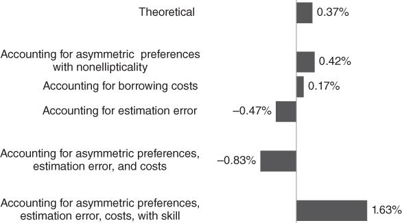
FIGURE 14.2 Outperformance of Leverage versus Concentration

THE BOTTOM LINE

It is apparent from Figure 14.2 that the outperformance of leverage over concentration, while theoretically sensible, does not always survive real‐world conditions. We relax the following constraints individually and then collectively:

• The assumption that returns are elliptically distributed and that investor preferences can be approximated by mean and variance, as well as the assumption that means and covariances can be estimated reliably.
• The assumption that investors can borrow at the risk‐free rate.
• The assumption that investors have homogeneous expectations for returns and covariances of asset classes, and that no investors have forecasting skill.

For the same level of risk, we find that the expected outperformance of the levered portfolio falls from 37 basis points in theory to –83 basis points after accounting for asymmetric preferences with nonelliptical distributions, and realistic borrowing costs. However, if we assume skill in forecasting returns, leverage outperforms concentration by 163 basis points despite all of these complexities.

The results we present in this chapter reflect a specific set of asset classes and assumptions, and do not hold universally. However, this framework could be customized easily to accommodate a wide range of assumptions and scenarios.

REFERENCES

1. H. Markowitz. 1952. “Portfolio Selection,” Journal of Finance, Vol. 7, No. 1 (March).
2. W. Sharpe. 1964. “A Theory of Market Equilibrium under Conditions of Risk,” Journal of Finance, Vol. 19, No. 3 (September).
3. J. Tobin. 1958. “Liquidity Preference as Behavior Towards Risk,” Review of Economic Studies, Vol. 25, No. 2 (February).

NOTES

1. The deviations should be calculated against the full‐sample mean. This way, the semistandard deviation collapses to the standard deviation if the return distribution is symmetric. We compute the semistandard deviations for each asset class, and then combine them with full‐sample correlations to arrive at a semi‐covariance matrix. We cannot compute semicorrelations because they would not be comparable to full‐sample correlations.

2. In Chapter 18 we define the kinked utility function more precisely.