CHAPTER 15
Rebalancing

THE CHALLENGE

In Chapter 2, we showed how to identify an efficient asset mix given assumptions about the expected returns, standard deviations, and correlations of asset classes. In Chapter 8, we introduced full‐scale optimization as a method to construct efficient portfolios when the assumptions necessary for mean‐variance analysis do not hold. Regardless of which method investors use to form portfolios, the portfolios become suboptimal almost immediately after implementation. Why? Price changes are not uniform across asset classes, so the portfolio weights drift away from the optimal targets over time. If there were no transaction costs, investors could trade daily, or even more often, to maintain the optimal weights. In practice, investors face a trade‐off: They must balance the transaction cost of restoring the optimal weights against the utility cost of remaining suboptimal.

Most investors employ simple heuristics to manage this trade‐off. Some implement calendar‐based rebalancing policies, in which they rebalance each month, quarter, or year. Others impose tolerance bands in which they rebalance when the exposure to any asset class drifts more than two percentage points from its target, for example. These approaches are better than not rebalancing at all. But they are arbitrary. Is total cost minimized by tolerance bands of one percentage point or two percentage points? Should equity asset classes have wider bands than fixed‐income asset classes? Should investors rebalance in periods when there has been little drift?

We propose that investors implement a rebalancing policy that minimizes explicitly the sum of transaction costs and suboptimality costs, including the expected future costs associated with each decision, at each point in time. Rebalancing is a multiperiod problem: A decision to rebalance today, or not, has implications for expected suboptimality and transaction costs in the future.

Sun, Fan, Chen, Schouwenaars, and Albota (2006) showed how to use dynamic programming to develop a rebalancing road map. This approach gives the optimal rebalancing decision for every possible combination of portfolio weights that may arise at each decision point during the investment horizon. They showed that this approach outperforms calendar and tolerance band approaches by reducing both transaction costs and suboptimality costs. Unfortunately, their dynamic programming solution suffers from the curse of dimensionality; it is intractable for portfolios with more than a few asset classes.

Markowitz and van Dijk (2003) introduced a quadratic heuristic to rebalance portfolios to capture changes in expected returns of assets through time. Kritzman, Myrgren, and Page (2009) applied this approach, which they call the Markowitz–van Dijk (MvD) heuristic, to the rebalancing problem. They show that the MvD solution is remarkably close to the dynamic programming solution for small numbers of assets, and that it scales manageably to several hundred assets. In this chapter, we begin with a simple example that illustrates the dynamic programming approach to highlight the intertemporal nature of the rebalancing problem. Then we show how the MvD heuristic can be used to rebalance portfolios in practice.

THE DYNAMIC PROGRAMMING SOLUTION

Dynamic programming was introduced by Bellman (1952) and has since been employed in a wide range of disciplines including biology, computer science, economics, and natural language processing. It is a method for solving a complex, multistage problem by breaking it down into an array of subproblems. Dynamic programming is computationally efficient because it saves the solution to each subproblem so it does not need to solve that subproblem again. It is often used in multiperiod optimization problems in which decisions in one period depend on the distribution of possible outcomes in future periods. In this context, Smith (1997) showed how to use dynamic programming to find the most desirable spouse. His results were highly intuitive. He showed that the optimal approach is to marry only a highly desirable partner in the early years, but if one does not come along, to lower one's standards as time runs out and desperation sets in.

To show how dynamic programming is applied to solve the rebalancing problem, consider a simple world with only two asset classes—stocks and bonds—and three potential return outcomes, as shown in Table 15.1. Specifically, there is a 25 percent chance that stocks and bonds will return 26 percent and 1 percent, respectively; a 25 percent chance that they will return –11 percent and 10 percent, respectively; and a 50 percent chance that they will both return 8 percent. Finally, assume that it costs 5 basis points to trade stocks and 7 basis points to trade bonds. Given these assumptions, an investor with log‐wealth utility will allocate 60 percent of the portfolio to stocks and 40 percent to bonds.¹ This portfolio offers the maximum expected utility of 0.0690.

TABLE 15.1 Return Distribution and Expected Log‐Wealth Utility for a 60/40 Portfolio

	Expected Returns (%)
Probability (%)	Stocks	Bonds	Log‐Wealth Utility	Product
25	26	1	ln[(1 + .26) × 60% + (1 + .01) × 40%]	0.0371
50	8	8	ln[(1 + .08) × 60% + (1 + .08) × 40%]	0.0385
25	−11	10	ln[(1 − .11) × 60% + (1 + .10) × 40%]	−0.0066
Weighted average	7.75	6.75		0.0690

Figure 15.1 shows all of the potential paths that the asset mix could take over two periods. At the end of the first period, there is a 25 percent chance that the mix would be 65/35, a 50 percent chance it would remain at 60/40 if both assets return 8 percent, and a 25 percent chance it would be 55/45. At the end of the second period, there is an even wider array of potential asset mixes. In the extremes, there is a 6.25 percent (25 percent × 25 percent) chance that the mix would be 70/30 and a 6.25 percent chance that it would be 50/50. At each point in this tree, the investor faces a decision: rebalance the portfolio to the optimal mix and incur transaction costs or don't rebalance, remain suboptimal, and thereby incur suboptimality costs.

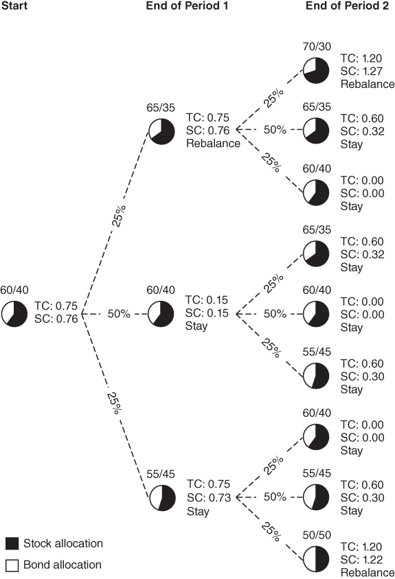
FIGURE 15.1 Trading and Suboptimality Costs over Two Periods

To implement dynamic programming we start by working backward from the end of period 2. Let us first consider the portfolio resulting from two successive 26 percent stock returns, which is 70 percent stocks and 30 percent bonds. We determine the utility of this portfolio by substituting a 70/30 stock/bond portfolio for the 60/40 portfolio in Table 15.1, which yields expected utility of 0.0689 percent. The certainty equivalent of the optimal 60/40 portfolio equals 1.071436 (or e^0.068881), whereas the certainty equivalent of a 70/30 portfolio equals 1.071308 (or e^0.068881).² Hence, the cost of suboptimality for the 70/30 portfolio equals the difference between these values: 127 basis points. This value is shown as the suboptimality cost (indicated by SC next to the 70/30 allocation at the end of period 2.

How does this suboptimality cost compare to the cost of rebalancing? The cost of restoring the optimal weights equals 120 basis points or (0.10 × 0.0005 + 0.10 × 0.0007), given that we need to trade 10 percent of the portfolio out of stocks at a cost of 5 basis points and into bonds at a cost of 7 basis points. This value is shown as the transaction cost (indicated by TC) next to the 70/30 allocation at the end of period 2. Therefore, given a 70/30 stock/bond portfolio at the end of period 2, we would choose to rebalance to the optimal mix because the cost of rebalancing is less than the suboptimality cost. We perform the same calculations to determine the optimal decision for the eight other possible portfolios at the end of period 2.

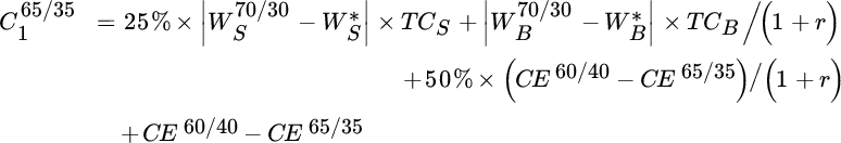
Next we step back to the end of period 1. Now there are only three portfolios to consider, but each portfolio leads to three additional possible portfolios at the end of period 2. To identify the optimal decision at the end of period 1, we must therefore account not only for the cost of each choice in period 1, but also for the present value of each decision's expected future costs in period 2. Consider, for example, the 65/35 portfolio at the end of period 1. The costs associated with retaining this portfolio, rather than rebalancing it, are given by Equation (15.1).

(15.1)

is the stock weight in the 70/30 portfolio, is the stock weight in the optimal portfolio (60 percent), is the transaction cost for stocks, is the bond weight in the 70/30 portfolio, is the bond weight in the optimal portfolio (40 percent), is the transaction cost for bonds, is the discount rate, is the certainty equivalent of the 60/40 (optimal) portfolio, and is the certainty equivalent of the 65/35 portfolio. We interpret this equation as follows:

• There is a 25 percent chance that this portfolio will lead to a 70/30 portfolio by the end of period 2. Given this outcome, we have just shown that it is optimal to rebalance to the 60/40 portfolio; hence, we must account for this potential future rebalancing cost, discounted back to the current period. This is the first line of Equation (15.1).
• There is a 50 percent chance that the portfolio weights will remain at 65/35, in which case we have shown it is optimal to retain these weights; hence, we must account for the potential future suboptimality of this 65/35 portfolio, discounted back to the current period. This is the second line of the equation.
• Finally, there is a 25 percent chance that the portfolio will shift to a 60/40 portfolio at the end of period 2. In this case there are neither suboptimality costs nor transaction costs to consider. Therefore, this outcome does not enter into the equation.
• In addition to these future costs, we must account for the fact that the 65/35 portfolio is suboptimal in the current period. This is the last line of the equation.

To determine the optimal choice for the 65/35 portfolio at the end of period 1, we compare the sum of these components from Equation (15.1) to the cost of rebalancing. The cost of rebalancing includes discounted future costs for the 60/40 portfolio. In this case, the rebalancing costs are lower than the suboptimality costs, so the optimal decision is to rebalance. We can repeat this entire exercise to determine the optimal choices given the other two portfolios at the end of period 1.

This illustration of dynamic programming highlights the intertemporal dependence of optimal rebalancing decisions. Unfortunately, as should be evident, this approach involves a large number of calculations. And this was just a simple example. In practice, investors must rebalance many asset classes over extended periods, allowing for return distributions with far more than three outcomes. For a portfolio of 10 asset classes, there are 4.2 trillion possible portfolios and over 10,000 trillion trillion calculations to perform. Notwithstanding advances in computing power, it is computationally impossible to derive the optimal decisions for a 10–asset class portfolio based on a search across 1 percent intervals, even if we employ an army of industrious interns.³ Dynamic programming suffers from the curse of dimensionality.

THE MARKOWITZ–VAN DIJK HEURISTIC

Unlike dynamic programming, the MvD approach is manageable even for relatively large numbers of asset classes. Like the dynamic programming solution, it seeks to account for both current and future costs associated with the decision to rebalance or to remain suboptimal. To implement it, we first define a cost function associated with rebalancing from a current portfolio to a possible new portfolio. This cost function is given by Equation (15.2).

(15.2)

is the cost of trading to a potential new portfolio. The terms and are the certainty equivalents of the optimal portfolio and the possible new portfolio, respectively. In practice we calculate mean‐variance utility rather than log‐wealth utility. The difference between these two terms is the suboptimality cost of the possible new portfolio. The weights we choose could be suboptimal, intentionally, because we wish to consider rebalancing trades that may only partially restore optimal weights but incur fewer transaction costs. The vectors and are the weights of the possible new and current portfolios, respectively, and is a vector of transaction costs for each asset class. This term captures the transaction cost of trading from the current portfolio to the possible new portfolio. The vector represents the weights of the optimal portfolio, and is a coefficient chosen to best approximate the true utility function. This last term is a quadratic function that approximates the discounted cost of future choices. We use Monte Carlo simulation to determine the value of .⁴ For a given set of current weights, , we identify a set of possible new portfolio weights, , that minimizes the cost function given by Equation (15.2).⁵ The optimal rebalancing decision is to rebalance to these weights.

To demonstrate this approach, we return to the moderate portfolio that we defined in Chapter 2. We evaluate the performance of four distinct approaches to rebalancing for the moderate portfolio:

• No rebalancing. This strategy is the easiest to implement. We simply allow the portfolio to drift throughout the investment horizon.
• Calendar‐based rebalancing. This strategy rebalances the portfolio back to the optimal targets on a fixed schedule, regardless of how much the weights have drifted. We consider monthly, quarterly, semiannual, and annual rebalancing schedules.
• Tolerance band rebalancing. This strategy rebalances the portfolio back to the optimal targets whenever any asset class weight breaches a predefined band around the optimal targets, regardless of how much time has elapsed since the last rebalance. We consider 1, 3, and 5 percent bands.
• Optimal MvD rebalancing. This strategy rebalances the portfolio each month to the weights that minimize the cost function given by Equation (15.2).

In practice, investors may consider other rebalancing strategies as well. For example, one approach is to use tolerance bands with varying sizes across asset classes. It is straightforward to evaluate any rebalancing strategy with this simulation framework.

Table 15.2 shows our transaction cost assumptions for each asset class. Investors who trade differently, or employ derivatives, may face a different set of transaction costs and should change these assumptions.

TABLE 15.2 Asset Class Transaction Costs

Asset Classes	Transaction Costs (basis points)
U.S. Equities	20
Foreign Developed Market Equities	35
Emerging Market Equities	60
Treasury Bonds	5
U.S. Corporate Bonds	50
Commodities	10
Cash Equivalents	3

To evaluate the performance of these strategies, we simulate 1,000 five‐year paths using Monte Carlo simulation, given the return and risk assumptions specified in Chapter 2. We measure the average suboptimality cost and transaction cost incurred by each strategy, as well as the annual turnover, average trade size, and average number of trades per year. Table 15.3 shows the average performance of each rebalancing strategy.

TABLE 15.3 Performance of Rebalancing Strategies

Rebalancing Strategy	Average Trades per Year	Average Trade Size (percent)	Annual Turnover (percent)	Transaction Costs (bps)	Suboptimality Costs (bps)	Total Costs (bps)
Optimal	12	0.26	21.36	3.9	1.5	5.4
1% bands	5	0.6	18.4	5.8	0.5	6.3
3% bands	1	1.4	7.4	2.3	3.4	5.8
5% bands	0.3	2.2	4.3	1.4	5.5	6.9
Monthly	12	0.3	28.3	8.9	0.0	8.9
Quarterly	4	0.6	16.4	5.2	1.2	6.4
Semiannually	2	0.8	11.6	3.7	1.8	5.5
Annually	1	1.2	8.3	2.6	3.1	5.7
No rebalance	0	0.0	0.0	0.0	17.0	17.0

The optimal rebalancing strategy offers the lowest overall cost of 5.4 basis points per year. As we should expect, the tolerance band rules incur more suboptimality costs and fewer transaction costs as the band size increases. The calendar‐based rules incur more suboptimality costs and fewer transaction costs as the frequency of rebalancing decreases. If we never rebalance the portfolio, we incur very high suboptimality costs but no transaction costs. Figures 15.2 and 15.3 present graphically the trade‐off between suboptimality and transaction costs.

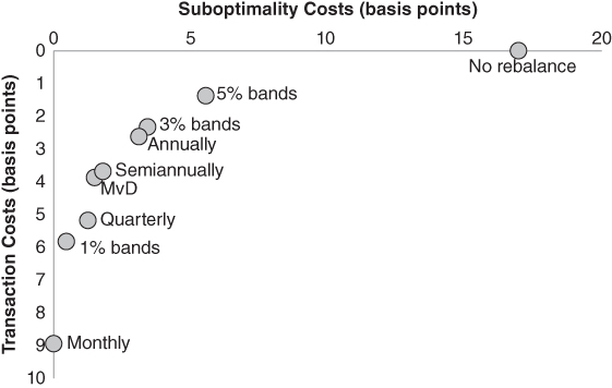
FIGURE 15.2 Performance of Rebalancing Strategies

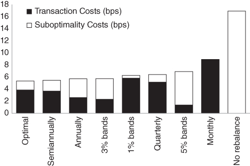
FIGURE 15.3 Performance of Rebalancing Strategies

In this example, we have assumed that all of the asset classes are liquid and can be traded at reasonable cost. In some instances, the portfolio will include illiquid asset classes that cannot be rebalanced. In these cases, we would adapt our simulation framework to rebalance the liquid asset classes while allowing the illiquid asset classes to drift. This approach has the benefit of accounting for the correlations between liquid and illiquid asset classes. To see why this is important, consider a portfolio that includes an illiquid private equity asset class that is correlated with liquid public equities. If the portfolio is overweight in public equities and underweight in private equity, the suboptimality cost of this distortion may be low because the asset classes are close substitutes for one another. With this insight we are able to rebalance more selectively and avoid excessive trading costs.

THE BOTTOM LINE

To develop an optimal rebalancing schedule, investors must evaluate the trade‐off between the transaction costs of restoring a portfolio's weights to their optimal targets and the suboptimality cost of retaining the current weights. They should also account for the future costs associated with each decision. In this chapter, we present an optimal rebalancing methodology and show that it outperforms simpler rebalancing rules.

REFERENCES

1. R. Bellman. 1952. “On the Theory of Dynamic Programming,” Proceedings of the National Academy of Sciences, Vol. 38, No. 8 (August).
2. M. Kritzman. 2008. “Rebalancing,” Economics and Portfolio Strategy (August).
3. M. Kritzman, S. Myrgren, and S. Page. 2009. “Optimal Rebalancing: A Scalable Solution,” Journal of Investment Management, Vol. 7, No. 1 (First Quarter).
4. H. Markowitz and E. L. van Dijk. 2003. “Single‐period Mean‐Variance Analysis in a Changing World,” Financial Analysts Journal, Vol. 59, No. 2 (March/April).
5. D. K. Smith. 1997. “Dynamic Programming: An Introduction,” Plus Magazine, accessed at: plus.maths.org/content/dynamic‐programming‐introduction.
6. W. Sun, A. Fan, L‐W. Chen, T. Schouwenaars, and M. Albota. 2006. “Optimal Rebalancing for Institutional Portfolios,” Journal of Portfolio Management, Vol. 32, No. 2 (Winter).

NOTES

1. We use log‐wealth utility in this example for simplicity. In practice, we assume mean‐variance utility, which approximates log‐wealth utility.

2. For more details on certainty equivalents, see Chapter 4 or the Appendix of Chapter 11.

3. For more details on the cure of dimensionality and optimal rebalancing, refer to Kritzman, Myrgren, and Page (2009).

4. We minimize cost at each decision point during the simulation. We continue to run simulations and change until we find its best‐performing value, which in this example is 0.30.

5. We could use a variety of optimization algorithms to minimize this cost function. We use the fmincon() function in Matlab.