Microsoft Excel has always provided users with a fairly comprehensive selection of formatting features. By applying different fonts, colors, borders, and patterns, or using conditional formatting and built-in styles, you can easily transform any raw and unfriendly worksheet data into a visually appealing and easy-to-understand document. Even if you don’t care about cell appearance and your only desire is to provide a no-frills data dump, chances are that before you share your worksheet with others you will spend ample time formatting cell values. For your raw data to be understood, you will definitely want to control the format of your numerical values, dates, and times.
To better highlight important information, you can apply conditional formatting with a number of visual features such as data bars, color scales, and icon sets. The sparkline feature allows you to place tiny charts in a cell to visually show trends alongside data. You can produce consistent-looking worksheets by using document themes and styles. When you select a theme, Excel automatically will make changes to text, charts, drawing objects, and graphics to reflect the theme you selected. By using Shape objects and SmartArt graphics layouts, you can bring different artistic effects to your worksheets.
This chapter assumes that you are already a master formatter and what really interests you is how the basic and advanced formatting features can be applied to your worksheets programmatically. So, let’s get to work.
This section focuses on cell value formatting that controls the relationship between the values that you enter in a worksheet cell and the cell’s format. Cell value formatting should always be attempted prior to cell appearance formatting. Always begin your formatting tasks by checking that Excel correctly interprets the values you entered or copied over from an external data source, such as a text file, an SQL Server, or a Microsoft Access database.
For example, when you copy data from an SQL Server and your data set contains date and time values separated by a space, such as 5/16/2016 11:00:04 PM, Excel displays the correct value in the formula bar, but displays 00:04.0 in the cell. When you activate the Format Cells dialog box, you will notice that Excel has applied the Custom format “mm:ss.0”, and if you take a look at the General format in the same dialog box, you will notice that the value was also converted to a serial number for date and time: 38853.95838. Or perhaps your data contains five-digit invoice numbers and you want to retain the leading zeros, which Excel suppresses by default.
When you enter data into a worksheet yourself, you are more likely to stop right away when Excel incorrectly interprets the data. When the data comes from an external source, it is much harder to pinpoint the cell formatting problems unless you run your custom VBA procedures that check for specific problems and automatically fix them when found. The meaning of your data largely depends on how Excel interprets your cell entries; therefore, to avoid confusing the end user, take the cell formatting control into your own hands.
Depending on how you have formatted the cell, the number that you actually see in a worksheet can differ from the underlying value stored by Excel. As you know, each new Excel worksheet will have its default cell format set to the built-in number format named “General.” In this format, Excel removes the leading and trailing zeros. For example, if you entered 08.40, Excel displays 8.4. In VBA, you can write the following statement to have Excel retain both zeros:
ActiveCell.NumberFormat = "00.00"
The NumberFormat property of the CellFormat object is used to set or return the format for a specific cell or cell range. The format code is the string displayed in the Format Cells dialog box (see Figure 18.1) or your custom string.
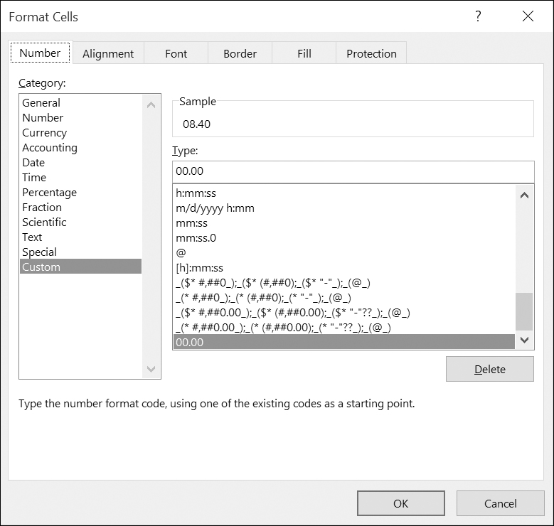
FIGURE 18.1. Format codes for your VBA procedures can be looked up in the Format Cells dialog box (choose Home | Format | Format Cells, or press Alt+H+O+E). The Custom category displays a list of ready-to-use number formats, and allows you to create a new format or edit the existing format code to suit your particular needs, such as 00.00 shown above.
If the number you entered has decimal places, Excel will only display as many decimal places as it can fit in the current column width. For example, if you enter 9.34512344443 in a cell that is formatted with the General format, Excel displays 9.345123 but keeps the full value you entered. When you widen the column, it will adjust the number of displayed digits. While determining the display of your number, Excel will also determine whether the last displayed digit needs to be rounded.
You can use the NumberFormat property to determine the format that Excel applied to cells. For example, to find out the format in the third column of your worksheet, you can use the following statement in the Immediate window:
?Columns(3).NumberFormat
If all cells in the specified column have the same format, Excel displays the name of the format, such as General, or the format code that has been applied, such as $#,##0.00. If different formatting is found in different cells of the specified column, Excel prints out Null in the Immediate window.
It is recommended that you apply the same number formatting for the entire column. Whether you are doing this programmatically or manually via the Excel user interface, the formatting can be applied before or after you enter the numbers. Excel will only apply number formatting to cells containing numeric values; therefore, you do not need to be concerned if the first cell in the selected column contains text that defines the column heading.
Because the NumberFormat property sets the cell’s number format by assigning a string with a valid format from the Format Cells dialog box, you can use the macro recorder to get the exact VBA statement for the format you would like to apply. For example, the following statements were generated by the macro recorder to format the values entered in cells D1 and E1
Range("D1").Select
Selection.NumberFormat = "#,##0"
and display a large number with the thousands separator (a comma) and with no decimal places.
Range("E1").Select
Selection.NumberFormat = "$#,##0.00"
displays a large number formatted as currency with the thousands separator and two decimal places.
The Custom category in the Format Cells dialog box (see Figure 18.1 earlier) lists many built-in custom formats that you can use in the NumberFormat property to control how values are displayed in cells. Also, you can create your own custom number format strings by using formatting codes as shown in Table 18.1.
TABLE 18.1. Number formatting codes |
Code |
Description |
0 |
Digit placeholder. Use it to force a zero. For example, to display .5 as 0.50, use the following VBA statement:
Selection.NumberFormat = "0.00"
or enter 0.00 in the Type box in the Format Cells dialog box. |
# |
Digit placeholder. Use it to indicate the position where the number can be placed. For example, the code #,### will display the number 2345 as 2,345. |
. |
Decimal placeholder. In the United States, a period is used as the decimal separator. In Germany, it is a comma. |
, |
Thousands separator (comma). In the United States, one thousand two hundred five is displayed as 1,205. In other countries, the thousands separator can be a period (e.g., Germany) or a space (e.g., Sweden). In the United States, placing a single comma after the number format indicates that you want to display numbers in thousands. To make it clear to the user that the number is in thousands, you may want to place the letter “K” after the comma:
Selection.NumberFormat = "#, ##0, K"
Use two commas at the end to display the number in millions:
Selection.NumberFormat = "#,##0.0,, "
To indicate that the number is in millions, add a backslash followed by “M”:
Selection.NumberFormat = "#,##0.0,,\M"
Or surround the letter “M” with double quotes:
Selection.NumberFormat = "#,##0.0,, ""M"""
This will cause the number 23093456 to appear as 23.1M. |
/ |
Forward slash character. Used for formatting a number as a fraction. For example, to format 1.25 as 1¼, use the following statement:
Selection.NumberFormat = "# ?/?"
|
_ |
The underscore character is used for aligning formatting codes. For example, to ensure that positive and negative numbers are aligned as shown below, apply the format as follows:
Selection.NumberFormat = "#,##0.00_);(#,##0.00)"
234.23
(234.12)
|
* |
The asterisk in a number format allows you to fill in the cell with the character that follows the asterisk. For example, the following VBA statement produces the output shown below:
Selection.NumberFormat = "*_0000"
_________1045
________23455
|
When working with cell formatting, keep in mind that number formats have four parts separated by semicolons. The first part is applied to positive numbers, the second to negative numbers, the third to zero, and the fourth to text. For example, take a look at the following VBA statement:
Range("A1:A4").NumberFormat = "#,##0;[red](#,#0);""zero"";@"
This statement tells Excel to format positive numbers with the thousands separator, display negative numbers in red and in parentheses, display the text “zero” whenever 0 is entered, and format any text entered in the cell as text. Make the following entries in cells A1:A4:
2870
-3456
0
Test text
When you apply the above format to cells A1:A4, you will see the cells formatted as shown below:
2,870
(3,456)
Zero
Test text
You can hide the content of any cell by using the following VBA statement:
Selection.NumberFormat = ";;;"
When the number format is set to three semicolons, Excel hides the display of the cell entry on the worksheet and in printouts. You can only see the actual value or text stored in the cell by taking a look at the Formula bar.
By using the number format codes, it is also possible to apply conditional formats with one or two conditions. Consider the following VBA procedure:
Sub FormatUsedRange()
ActiveSheet.UsedRange.Select
Selection.SpecialCells(xlCellTypeConstants, 1).Select
Selection.NumberFormat = "[<150][Red];[>250][Green];[Yellow]"
End Sub
This procedure tells Excel to select all the values in the used range on the active sheet and display them as follows: values less than 150 in red, values over 250 in green, and all the other values in the range from 150 to 250 in yellow. Excel supports eight popular colors: [white], [black], [blue], [cyan], [green], [magenta], [red], and [yellow], as well as 56 colors from the predefined color palette that you can access by indicating a number between 1 and 56, such as [Color 11] or [Color 32]. Be sure to use closed brackets to enclose conditions and colors.
Later in this chapter we will learn how to use VBA to perform more advanced conditional formatting.
In addition to the NumberFormat property, Excel VBA has a Format function that you can use to apply a specific format to a variable. For example, take a look at the following procedure that formats a number prior to entering it in a worksheet cell:
Sub FormatVariable()
Dim myResult, frmResult
myResult = "1435.60"
frmResult = Format(myResult, "Currency")
Debug.Print frmResult
ActiveSheet.Range("G1").FormulaR1C1 = frmResult
End Sub
When you run the FormatVariable procedure, cell G1 in the active worksheet will contain the entry $1,435.60. The Format function specifies the expression to format (in this case the expression is the name of the variable that stores a specified value) and the number format to apply to the expression. You can use one of the predefined number formats such as: “General”, “Currency”, “Standard”, “Percent”, and “Fixed”, or you can specify your custom format using the formatting codes from Table 18.1. For example, the following statement will apply number formatting to the value stored in the myResult variable and assign the result to the frmResult variable:
frmResult = Format(myResult, "#.##0.00")
For more information about the Format function and the complete list of formatting codes, refer to the online help.
To check whether the cell value is a number, use the IsNumber function as shown below:
MsgBox Application.WorksheetFunction.IsNumber(ActiveCell.Value)
If the active cell contains a number, Excel returns True; otherwise, it returns False.
NOTE |
To use an Excel function in VBA, you must prefix it with “Application.WorksheetFunction.” The WorksheetFunction property returns the WorksheetFunction object that contains functions that can be called from VBA. |
To format a cell as a text string, use the following VBA statement:
Selection.NumberFormat = "@"
To find out if a cell value is a text string, use the following statement:
MsgBox Application.WorksheetFunction.IsText(ActiveCell.Value)
Use the UCase function to convert a cell entry to uppercase:
Range("K3").value = UCase(ActiveCell.Value)
Use the LCase function to convert a cell entry to lowercase if the cell is not a formula:
If not Range(ActiveWindow.Selection.Address).HasFormula then
ActiveCell.Value = LCase(ActiveCell.Value)
End If
Use the Proper function to capitalize the first letter of each word in a text string:
ActiveCell.Value = Application.WorksheetFunction.Proper(ActiveCell.Value)
Use the Replace function to replace a specified character within text. For example, the following statement replaces a space with an underscore (_) in the active cell:
ActiveCell.Value = Replace(ActiveCell.Value, " ", "_")
To ensure that the text entries don’t have leading or trailing spaces, use the following VBA functions:
• LTrim—Removes the leading spaces
• RTrim—Removes the trailing spaces
• Trim—Removes both the leading and trailing spaces
For example, the following statement written in the Immediate window will remove the trailing spaces from the text found in the active cell:
ActiveCell.value = RTrim(ActiveCell.value)
Use the Font property to format the text displayed in a cell. For example, the following statement changes the font of the selected range to Verdana:
Selection.Font.Name = "Verdana"
You can also format parts of the text in a cell by using the Characters collection. For example, to display the first character of the text entry in red, use the following statement:
ActiveCell.Characters(1,1).Font.ColorIndex = 3
Microsoft Excel stores dates as serial numbers. In the Windows operating system, the serial number 1 represents January 1, 1900. If you enter the number 1 in a worksheet cell and then format this cell as Short Date using the Number Format drop-down in the Number section of the Ribbon’s Home tab, Excel will display the date formatted as 1/1/1900 and will store the value of 1 (you can check this out by looking at the General category in the Format Number dialog box). By storing dates as serial numbers, Excel can easily perform date calculations.
To apply a date format to a particular cell or range of cells using VBA, use the NumberFormat property of the Range object, like this:
Range("A1").NumberFormat = "mm/dd/yyyy"
Formatting codes for dates and times are listed in Table 18.2.
TABLE 18.2. Date and time formatting codes |
Code |
Description |
D |
Day of the month. Single-digit number for days from 1 to 9. |
Dd |
Day of the month (two-digit). Leading zeros appear for days from 1 to 9. |
ddd |
A three-letter day of the week abbreviation (Mon, Tue, Wed, Thu, Fri, Sat, and Sun). |
m |
Month number from 1 to 12. Zeros are not used for single-digit month numbers. |
mm |
Two-digit month number. |
mmm |
Three-letter month name abbreviation (e.g., Jan, Jun, Sep). |
yy |
Two-digit year number (e.g., 13). |
yyyy |
Four-digit year number (e.g., 2016). |
h |
The hour from 0 to 23 (no leading zeros). |
hh |
The hour from 0 to 23 (with leading zeros). |
:m |
The minute from 0 to 59 (no leading zeros). |
:mm |
The minute from 0 to 59 (with leading zeros) |
:s
:s.0
:s.00 |
The second from 0 to 59 (no leading zeros).
To add tenths of a second, follow this with a period and a zero (.0), and to add hundredths of a second, follow this code with a period and two zeros (.00). |
:ss
:ss.0
:ss.00 |
The second from 0 to 59 (with leading zeros).
To add tenths of a second, follow this code with a period and a zero (.0), and to add hundredths of a second, follow this code with a period and two zeros (.00). |
AM/PM
am/pm
A/P
a/p |
Use for a 12-hour clock, with AM or PM.
Use for a 12-hour clock, with am or pm.
Use for a 12-hour clock, with A or P.
Use for a 12-hour clock, with a or p. |
[ ] |
Bracket the time component (hour, minute, second) to prevent Excel from rolling over hours, minutes, or seconds when they hit the 24-hour mark (hours become days) or the 60 mark (minutes become hours, seconds become minutes). For example, to display time as 25 hours, 59 minutes, and 12 seconds use the following format code: [hh]:[mm]:ss. |
The following VBA procedure applies a date format to the Inspection Date column in Figure 18.2.
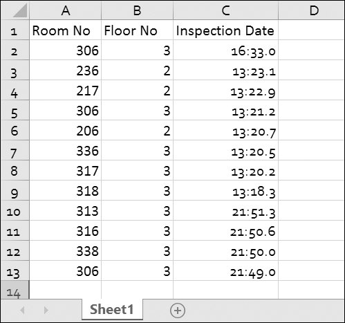
FIGURE 18.2. A worksheet with an unformatted Inspection Date column.
Sub FormatDateFields()
Dim wks As Worksheet
Dim cell As Range
Set wks = ActiveWorkbook.ActiveSheet
For Each cell In wks.UsedRange
If cell.NumberFormat = "mm:ss.0" Then
cell.NumberFormat = "m/dd/yyyy h:mm:ss AM/PM"
End If
Next
End Sub
After running the above procedure, the cells in column C are displayed as shown in Figure 18.3.

FIGURE 18.3. The Inspection Date column has been formatted with a VBA procedure.
To speed up your worksheet formatting tasks you can apply formatting to entire rows and columns instead of single cells. The best way to find the required VBA statement is by using the macro recorder (choose Developer | Record Macro). Keep in mind that Excel will record more code than is necessary for your specific task and you’ll need to clean it up before copying it to your VBA procedure. For example, here’s the recorded code for setting the horizontal alignment of data in Row 7:
Rows("7:7").Select
Range("D7").Activate
With Selection
.HorizontalAlignment = xlRight
.VerticalAlignment = xlBottom
.WrapText = False
.Orientation = 0
.AddIndent = False
.IndentLevel = 0
.ShrinkToFit = False
.ReadingOrder = xlContext
.MergeCells = False
End With
To set the horizontal alignment for Row 7, you can write a single VBA statement like this:
Rows(7).HorizontalAlignment = xlRight
You can use the macro recorder to help you find out the names of properties that should be used to turn on or off a specific formatting feature. Once you know the property and the required setting, you can write your own short statement to get the job done.
Here are some VBA statements that can be used to format columns and rows:
Formatting Columns and Rows |
VBA Statement |
To format column D as a date using the NumberFormat property: |
Columns("D").NumberFormat = "mm/dd/yyyy"
|
To format column G as currency: |
Columns("G").NumberFormat = "$###,##0.00"
|
To format column G as currency using the Style property: |
Columns("G").Style = "Currency"
|
To set column width or row height: |
Columns(2).ColumnWidth = 21.5
Rows(2).RowHeight = 55.55
|
To auto-fit column width or row height: |
Columns(2).AutoFit
Rows(2).Autofit
|
To apply bold font to the first row: |
Rows(1).Font.Bold = True
|
To right-align data in row 1: |
Rows(1).HorizontalAlignment = xlRight
|
To center data in column B: |
Columns("B").HorizontalAlignment = xlCenter
|
To set the background of the column where the active cell is located to yellow: |
Columns(ActiveCell.Column). interior.color = vbYellow
|
To check the width of a column, use the ColumnWidth method: |
MsgBox Columns(ActiveCell. Column).ColumnWidth
|
To auto-fit all rows and columns: |
ActiveSheet.Cells.EntireRow. AutoFit
ActiveSheet.Cells.EntireColumn.AutoFit
|
Headers and footers are made of three sections each: LeftHeader, CenterHeader, and RightHeader, and LeftFooter, CenterFooter, and RightFooter. Using the special formatting codes shown in Table 18.3, you can customize your worksheet’s header or footer according to your needs.
TABLE 18.3. Header and footer formatting codes |
Format Code |
Description |
&D |
Prints the current date |
&T |
Prints the current time |
&F |
Prints the name of the workbook |
&A |
Prints the name of the sheet tab |
&P |
Prints the page number |
&P+number |
Prints the page number plus the specified number |
&P–number |
Prints the page number minus the specified number |
&N |
Prints the total number of pages in the workbook |
&Z |
Prints the workbook’s path |
&G |
Inserts an image |
&& |
Prints a single ampersand |
&nn |
Prints the characters that follow in the specified font size in points |
&color |
Prints the characters in the specified color using the hexadecimal color value |
&”fontname” |
Prints the characters that follow in the specified font |
&L |
Left-aligns the characters that follow |
&C |
Centers the characters that follow |
&R |
Right-aligns the characters that follow |
&B |
Turns bold printing on or off |
&I |
Turns italic printing on or off |
&U |
Turns underline printing on or off |
&E |
Turns double-underline printing on or off |
&S |
Turns strikethrough printing on or off |
&X |
Turns superscript printing on or off |
&Y |
Turns subscript printing on or off |
Here are several VBA statements that demonstrate applying custom formatting to a header or footer:
Formatting Headers and Footers |
VBA Statement (enter on one line) |
To create a two-line header with bold text in the first line and italic text in the second line: |
ActiveSheet.PageSetup.LeftHeader = "&BYour Company Name" & Chr(13) & "&IYour Company Department"
|
To place the workbook creation date in the footer: |
ActiveSheet.PageSetup.RightFooter = "Created on: " & ActiveWorkbook.BuiltinDocumentProperties
("Creation Date")
|
To place a cell’s contents in the header: |
ActiveSheet.PageSetup.CenterHeader = ActiveSheet.Cells(2,2).value
|
To insert the filename and path in the footer: |
ActiveSheet.PageSetup.CenterFooter = ActiveWorkbook.FullName
|
To place text in the header using Arial Narrow font and italic formatting, with the last word in bold, italic, and red: |
ActiveSheet.PageSetup.CenterHeader = "&""ArialNarrow""&IYour text goes here &I&B&KFF0000now."
|
To remove the formatting and text entries from the center header: |
ActiveSheet.PageSetup.CenterHeader = ""
|
NOTE |
If you need to use a different date format in your header or footer than the date format shown in the Regional settings of the Windows Control panel, use the Format function to specify the date format string you want to use:
ActiveSheet.PageSetup.RightFooter = Format(Date, "mm-dd-yyyy")
The above statement inserts in the right footer a current system date returned by the Date function. The date is formatted as a two-digit month number followed by a dash, two-digit day number followed by a dash, and four-digit year number (see Table 18.2 for the explanation of date and time formatting codes). |
As mentioned earlier, adding cosmetic touches to your worksheet such as fonts, color, borders, shading, and alignment should be undertaken after applying the required formatting to numbers, dates, and times. Formatting cell appearance makes your worksheet easier to read and interpret. By applying borders to cells, and with the clever use of font colors, background shading, and patterns, you can draw the reader’s attention to particularly important information.
Use the Font object to change the font format in VBA. You can easily apply multiple format properties using the With…End With statement block shown below:
Sub ApplyCellFormat()
With ActiveSheet.Range("A1").Font
.Name = "Tahoma"
.FontStyle = "italic"
.Size = 14
.Underline = xlUnderlineStyleDouble
.ColorIndex = 3
End With
End Sub
The ColorIndex property refers to the 56 colors that are available in the color palette. Number 3 represents red. The following procedure prints a color palette to the active sheet:
Sub ColorLoop()
Dim r As Integer
Dim c As Integer
Dim k As Integer
k = 0
For r = 1 To 8
For c = 1 To 7
Cells(r, c).Select
k = k + 1
ActiveCell.Value = k
With Selection.Interior
.ColorIndex = k
.Pattern = xlSolid
End With
Next c
Next r
End Sub
To change the background color of a single cell or a range of cells, use one of the following VBA statements:
Selection.Interior.Color = vbBlue
Selection.Interior.ColorIndex = 5
To change the font color, use the following VBA statement:
Selection.Font.Color = vbMagenta
The font can be made bold, italic, or underlined or a combination of the three using the following With…End With block statement:
With Selection.Font
.Italic = True
.Bold = True
.Underline = xlUnderlineStyleSingle
End With
To apply borders to your cells and ranges in VBA, use the following statement examples:
Selection.BorderAround Weight:=xlMedium, ColorIndex:=3
Selection.BorderAround Weight:=xlThin, Color:=vbBlack
The BorderAround method of the Range object places a border around all edges of the selected cells. The following xlBorderWeightEnumeration constants can be used to specify the thickness weight of the border: xlHairline, xlMedium, xlThick, and xlDash. When specifying border color, you can use either ColorIndex or Color but not both.
Instead of specifying the thickness of the border, you may want to use LineStyle as in the following example:
Selection.BorderAround LineStyle:=xlDashDotDot, Color:=vbBlack
You can use any of the following xlLineStyle enumeration constants:
• xlContinuous
• xlDash
• xlDashDot
• xlDashDotDot
• xlDot
• xlDouble
• xlLineStyleNone
• xlSlantDashDot
Use xlLineStyleNone to clear the border.
VBA has a Borders collection that contains the four borders of a Range or Style object. To set just a bottom border of cells A1:C1, use the following statement:
ActiveSheet.Range("A1:C1").Borders(xlEdgeBottom).Weight = xlThick
You may specify any of the following border types:
• xlDiagonalDown
• xlDiagonalUp
• xlEdgeBottom
• xlEdgeLeft
• xlEdgeRight
• xlEdgeTop
• xlEdgeHorizontal
• xlEdgeVertical
You can change the appearance of cells by specifying the horizontal or vertical alignment:
Selection.HorizontalAlignment = xlCenter
Selection.VerticalAlignment = xlTop
The value of the HorizontalAlignment property can be one of the following constants:
• xlCenter
• xlDistributed
• xlJustify
• xlLeft
• xlRight
The VerticalAlignment property can be one of the following constants:
• xlBottom
• xlCenter
• xlDistributed
• xlJustify
• xlTop
To remove cell formatting, use the ClearFormats method of the Range object. This method restores the formatting to the original General format without removing the cell’s content. To remove the content of the cell, use the ClearContents method.
Let’s focus on how you can use VBA with the enhanced formatting features that are available in the Styles group on the Ribbon’s Home tab and in the Themes group of the Page Layout tab. We will work with the FormatConditions collection of the Range object and explore the conditional formatting tools: data bars, color scales, and icon sets. Then we’ll look at how sparklines can be used to enhance your worksheets. We will also take a look at document themes that can be applied to a workbook, and see how they affect another formatting feature—styles.
To help you automatically highlight important parts of your worksheet, Excel provides a feature known as conditional formatting. This feature allows you to set a condition (a formatting rule), and specify the type of formatting that should be applied to cells and ranges when the condition is met. For example, you can use conditional formatting to apply different background colors, fonts, or borders to a cell based on its value. The Conditional Formatting feature provides users with various types of common rules and formatting tools such as data bars, color scales, and icon sets that make it easy to highlight certain worksheet data. For example, you can highlight the top or bottom 10% of values, locate duplicate or unique values, or indicate values above or below the average.
Excel allows you to specify an unlimited number of conditional formats and refer to ranges in other worksheets when using conditional formats. The Conditional Formatting Rules Manager shown in Figure 18.4 simplifies the creation, modification, and removal of conditional rules. All conditional formatting features that are available in the Excel application window can be accessed via VBA.

FIGURE 18.4. To activate the Conditional Formatting Rules Manager, choose Home | Conditional Format-ting | Manage Rules.
To create a new conditional formatting rule, click the New Rule button in the Conditional Formatting Rules Manager dialog box. You will see the list of built-in rules that you can select from, as shown in Figure 18.5.
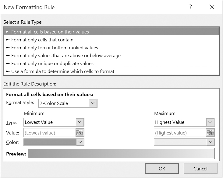
FIGURE 18.5. Creating a new conditional format using the Excel built-in dialog. This window appears after choosing the New Rule button in the Conditional Formatting Rules Manager shown in Figure 18.5, or choosing Home | Conditional Formatting | New Rule.
In VBA, use the Add method of the FormatConditions collection to create a new rule. For example, to format cells containing “Qtr” in the text string, enter the following procedure in a standard module and then run it:
Sub FormatQtrText()
With ActiveSheet.UsedRange
.FormatConditions.Delete
.FormatConditions.Add Type:=xlTextString, String:="Qtr", TextOperator:=xlContains
.FormatConditions(1).Interior.Color = RGB(123, 130, 0)
End With
End Sub
Notice that before creating and applying a new conditional format to a range of cells, it’s a good idea to delete the existing format condition from the selection using the Delete method. The Add method that is used to add a new condition requires at least the Type argument that specifies whether the conditional format is based on a cell value or an expression. Use the xlFormatConditionType enumeration constants listed in Table 18.4 to set the condition type. For example, to format cells that contain dates, use the xlTimePeriod constant in the Type argument, and specify the DateOperator using one of the following constants: xlToday, xlYesterday, xlTomorrow, xlLastWeek, xlThisWeek, xlNextWeek, xlLast7Days, xlLastMonth, xlThisMonth, or xlNextMonth:
Selection.FormatConditions.Add Type:=xlTimePeriod, DateOperator:=xlLast7Days
TABLE 18.4. Conditional format Type settings (xlFormatConditionType enumeration) |
Constant |
Description |
xlAboveAverageCondition |
Above/below average condition:
With Selection
.FormatConditions.Delete
.FormatConditions.AddAboveAverage
.FormatConditions(1).AboveBelow = xlAboveAverage
.FormatConditions(1).Font.Bold = True
End With
|
xlBlanks
Condition |
Format cells that contain blanks:
With Selection
.FormatConditions.Add Type:=xlBlanksCondition
End With
|
xlCellValue |
Format a cell value:
With Selection
.FormatConditions.Add Type:=xlCellValue,
Operator:=xlLess
Formula1:="=2000"
.FormatConditions(1).NumberFormat = "#, ##0"
End With
You can use the following constants in the Operator argument: xlBetween, xlEqual, xlGreater, xlGreaterEqual, xlLess, xlLessEqual, xlNotBetween, or xlNotEqual. |
| |
To specify the numeric value for the operator, use the Formula1 argument. The xlBetween and xlNotBetween operators require that you also specify a second value in Formula2. |
xlColorScale |
Format color scale:
If Selection.FormatConditions(1).Type = 3 Then
MsgBox "Formatted with " & "ColorScale conditional format."
End If
|
xlDataBar |
Format data bar:
If Selection.FormatConditions(1).Type = 4 Then
MsgBox "Formatted with " & "DataBar conditional format."
End If
|
xlErrors
Condition |
Format cells that contain errors:
Selection.FormatConditions.Add Type:=xlErrorsCondition
|
xlExpression |
Expression to specify a custom formula that identifies the cells that the conditional format applies to. For example, the following procedure changes the background color of alternate rows in the used range:
Sub HighlightAltRows()
With ActiveSheet.UsedRange
.FormatConditions.Add Type:=xlExpression, Formula1:="=MOD(ROW(),2)=0"
.FormatConditions(1).Interior.ColorIndex = 6
End With
End Sub
To highlight every third row, use the formula:
= MOD(ROW(),3)= 0
|
xlIconSet |
Format icon set:
If Selection.FormatConditions(1).Type = 6 Then
MsgBox "Formatted with " & "IconSet conditional format."
End If
|
xlNoBlanks
Condition |
Format cells that do not contain blanks:
Sub HighlightNonEmptyCells()
Range("A1:B12").Select
Selection.FormatConditions.Add Type:=xlNoBlanksCondition
With Selection.FormatConditions(1).Interior
.ThemeColor = xlThemeColorAccent4
.TintAndShade = 0.399945066682943
End With
End Sub
|
xlNoErrors
Condition |
Format cells that do not contain errors:
Sub HighlightCellsWithNoErrors()
Range("F1:F7").Select
Selection.FormatConditions.Add Type:=xlNoErrorsCondition
With Selection.FormatConditions(1).Interior
.ThemeColor = xlThemeColorAccent4
.TintAndShade = 0.399945066682943
End With
End Sub
Before running the above procedure, enter any number in cell F1, and enter zero (0) in cell F2. In cell F3 enter the following formula: =F1/F2. Because there is no division by zero, Excel will display the following error code: #DIV/0! When you run the procedure, all cells in the selected range except for cell F2 will be shaded with the specified color. |
xlTextString |
Format cells that contain text:
With ActiveSheet.UsedRange
.FormatConditions.Add Type:=xlTextString, String:="es", TextOperator:=xlContains
.FormatConditions(1).Font.Bold = True
End With
Other text operators you can use: xlBeginsWith, xlDoesNotContain, and xlEndsWith. |
xlTimePeriod |
Format cells that contain dates:
With ActiveSheet.UsedRange
.FormatConditions.Add Type:=xlTimePeriod, DateOperator:=xlLastMonth
.FormatConditions(1).Interior.ColorIndex = 6
End With
Other date operators you can use: xlToday, xlYesterday, xlTomorrow, xlLastWeekn, xlThisWeek, xlNextWeek, xlLast7Days, xlThisMonth, and xlNextMonth. |
xlTop10 |
Format 10 top values:
With Selection
.FormatConditions.AddTop10
.FormatConditions(1).TopBottom = xlTop10Top
.FormatConditions(1).Value = 5
.FormatConditions(1).Percent = False
.FormatConditions(1).Interior.Color = RGB(255,0,0)
End With
|
xlUniqueValue |
Format unique values:
With Selection
.FormatConditions.AddUniqueValues
.FormatConditions(1).DupeUnique = xlUnique Formula1:="=200"
End With
By replacing the xlUnique constant with xlDuplicate, you can select duplicate values. |
You can apply multiple conditional formats to a cell. For example, you can apply a conditional format to make the cell bold, and then another one to make a red border around the cell. Because these two formats do not conflict with one another, they can both be applied to the same cell. However, if you create another format that tells Excel to apply a blue border to the cell, this rule will not be applied because it conflicts with the previous rule that told Excel to apply the red border. In order to control multiple conditions applied to a range of cells, Excel uses rule precedence. When rules conflict with one another, Excel applies the rule that is higher in precedence. Rules are evaluated in order of precedence by how they are listed in the Conditional Formatting Rules Manager dialog box. In VBA, this is controlled by the Priority property of the FormatConditions object. For example, to assign a second priority to the first rule, use the following statement:
Range("B2:B17").FormatConditions(1).Priority = 2
You can make the rule the lowest priority with the following statement:
Range("B2:B17").FormatConditions(1).SetLastPriority
NOTE |
In cases where the same format is applied both manually and via conditional formatting to a range of cells, the conditional formatting rule takes precedence over the manual format. Formats applied manually are not considered when determining conditional formatting rule precedence and do not appear in the Conditional Formatting Rules Manager dialog box. |
You can use the following statement to delete all rules applied to a specific range of cells:
Range("B2:B17").FormatConditions.Delete
To delete a particular rule, refer to its index number before calling the Delete method of the FormatConditions collection:
Range("B2:B17").FormatConditions(2).Delete
The data visualization tool known as the data bar allows users to easily see how data values relate to each other. Data bars can be added via conditional formatting using the New Formatting Rule dialog box in Figure 18.6, or by a VBA procedure.
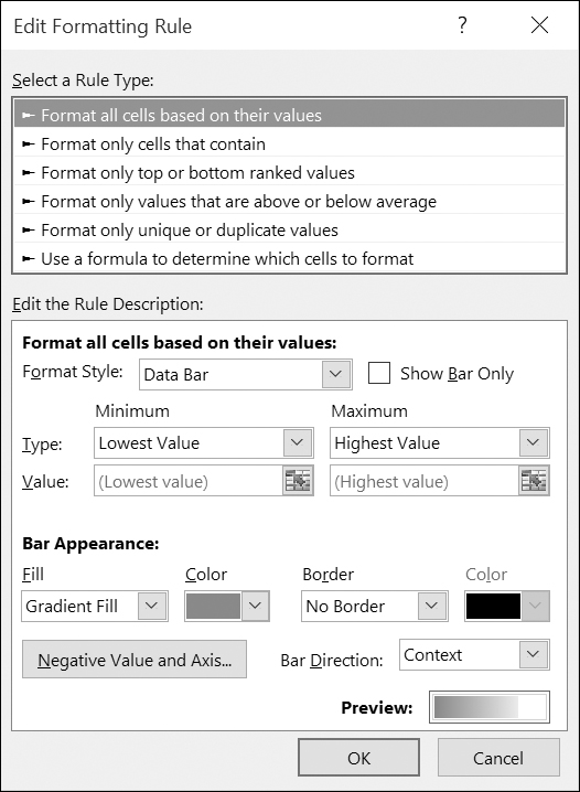
FIGURE 18.6. The New Formatting Rule dialog box can be accessed from the Ribbon by choosing Home | Conditional Formatting | Data Bars | More Rules.
Excel draws data bars proportionally according to their values. Thanks to this feature, data bars can be used to compare values. When you select the lowest value in the Type drop-down (see Figure 18.6), the data bar will not be drawn. When you select maximum value, Excel will draw a bar that covers the entire cell.
You can easily format the bar appearance with additional formatting options such as solid fills and borders. Thanks to this feature, you can see which cell has the highest value. However, keep in mind that applying a solid fill to a data bar may make some portions of the text harder to read, especially when using darker colors.
In VBA, you can create a data bar formatting rule by using the AddDatabar or Add method of the FormatConditions collection, as shown below:
Sub FormatWithDataBars()
With Range("B2:E6").FormatConditions
.AddDatabar
.Add Type:=xlDatabar, Operator:=xlGreaterEqual, Formula1:="200"
End With
End Sub
This procedure will place a blue bar in the worksheet cells, as illustrated in Figure 18.7. Notice that the length of the data bar corresponds to the cell’s value. If you change or recalculate the worksheet data, the data bar is automatically reapplied to the specified range. Instead of using the Lowest and Highest values to specify the Shortest and Longest bars in Figure 18.6, you can specify that the bar be based on numbers, percentages, formulas, or percentiles. For example, you can use the following statements to change the color, type, and threshold parameters of the data bar:
set mBar = Selection.FormatConditions.AddDatabar
mBar.MinPoint.Modify NewType:=xlConditionValuePercentile, NewValue:=20
mBar.MaxPoint.Modify NewType:=xlConditionValuePercentile, NewValue:=80
mBar.BarColor.ColorIndex = 7
In the previous statements, the MinPoin and MaxPoint properties of the DataBar object are used to set the values of the shortest and longest bars of a range of data, and the BarColor property is used to modify the color of the bars in the data bar conditional format.

FIGURE 18.7. A worksheet shown with the new data bar formatting.
You can create special visual effects in your worksheet by selecting a range of values and applying a color scale. Color scales use cell shading to help you understand variation in your data. When you apply a color scale conditional format via the user interface (Home | Conditional Formatting | Color Scales | More Rules) or from your VBA procedure, Excel uses the lowest, highest, and midpoint values in the range to determine the color gradients. You can apply a two-color or a three-color scale to your data, as shown in Figure 18.8.
To create a color scale conditional formatting rule in VBA, use the AddColorScale or Add method of the FormatConditions collection:
set cScale = Selection.FormatConditions.AddColorScale (ColorScaleType:=2)
The previous statement creates a two-color ColorScale object in the selected worksheet cells.
To change the minimum threshold to green and the maximum threshold to blue, use the following statements:
cScale.ColorScaleCriteria(1).FormatColor.Color = RGB(0, 255, 0)
cScale.ColorScaleCriteria(2).FormatColor.Color = RGB(0, 0, 255)
For darker color scales, it makes sense to change the font color to white:
Selection.Font.ColorIndex = 2
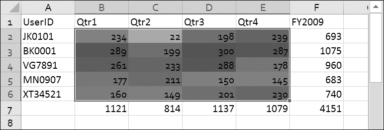
FIGURE 18.8. This worksheet was reformatted using a two-color color scale conditional format.
As with a data bar, you can change the type of threshold value for a color scale to a number, percent, formula, or percentile.
To create striking visual effects, try applying both data bar and color scale conditional formatting to the same range of data.
Icon sets are another visualization feature. By using icon sets, you can place icons in cells to make your data more comprehensive and visually appealing. Icon sets allow users to easily see the relationship between data values as well as recognize trends in the data.
To view the available icon choices, shown in Figure 18.9, choose Home | Conditional Formatting | Icon Sets.

FIGURE 18.9. You can select from a wide variety of built-in icons.
Each icon in an icon set represents a range of values. For example, in the three-icon set “3 Symbols (Circled)” shown in Figures 18.9 and 18.10, Excel uses the check mark symbol in a green circle for values that are greater than or equal to 67%, an exclamation point in an orange circle for values that are less than 67% and greater than or equal to 33%, and an X symbol in a red circle for values that are less than 33%.

FIGURE 18.10. You can display each icon according to the rules set in the New Formatting Rule dialog box.
Icon sets have become a very effective highlighting tool, thanks to the ability to apply icons only to specific cells instead of the entire range of cells. You can hide the icon for cells that meet the specified criteria by selecting No Cell Icon from the icon drop-down, as shown in Figure 18.11.

FIGURE 18.11. Excel allows users to hide icons for cells that meet the specified criteria.
The Icon Style drop-down also allows you to select four- and five-icon sets. These sets display each icon according to which quartile or quintile the value falls into.
You may change the default threshold value and its type (number, percent, formula, or percentile) for each icon in an icon set by editing the formatting rule using the dialog box shown in Figure 18.11 or with a VBA procedure as demonstrated in Hands-On 18.1.
NOTE |
Icons can be made larger or smaller by increasing or decreasing the font size. |
In VBA, the IconSet object in the IconSets collection represents a single set of icons. To create a conditional formatting rule that uses icon sets, use the IconSetCondition object. You can add criteria for an icon set conditional formatting rule with the IconCriteria collection. The following VBA procedure applies an icon set conditional formatting rule to a range of cells. The final result of this procedure is depicted in Figure 18.12.

|
Please note files for the “Hands-On” project may be found on the companion CD-ROM. |
1. Copy the Chap18_VBAExcel2016.xlsm file from the Companion CD to your VBAExcel2016_ByExample folder.
2. Open the C:\VBAExcel2016_ByExample\Chap18_VBAExcel2016.xlsm workbook and select Sheet3.
3. Switch to the Visual Basic Editor screen and insert a new module into VBAProject (Chap18_VBAExcel2016.xlsm).
4. In the module’s Code window, enter the following IconSetRules procedure:
Sub IconSetRules()
Dim iSC As IconSetCondition
Columns("C:C").Select
With Selection
.SpecialCells(xlCellTypeConstants, 23).Select
.FormatConditions.Delete
.NumberFormat = "$#,##0.00"
Set iSC = Selection.FormatConditions.AddIconSetCondition
iSC.IconSet = ActiveWorkbook.IconSets(xl3Symbols)
End With
End Sub
This procedure applies the currency format to the cell values in column C and clears the selected range from the conditional format that may have been applied earlier. Next, the AddIconSetCondition method is used to create an icon set conditional format for the selected range of cells.
In Step 5, when you run the procedure in step mode by pressing the F8 key, you will notice colored circles being applied to the cells. The next statement actually changes the default icon set to xl3Symbols as shown in Figure 18.12.
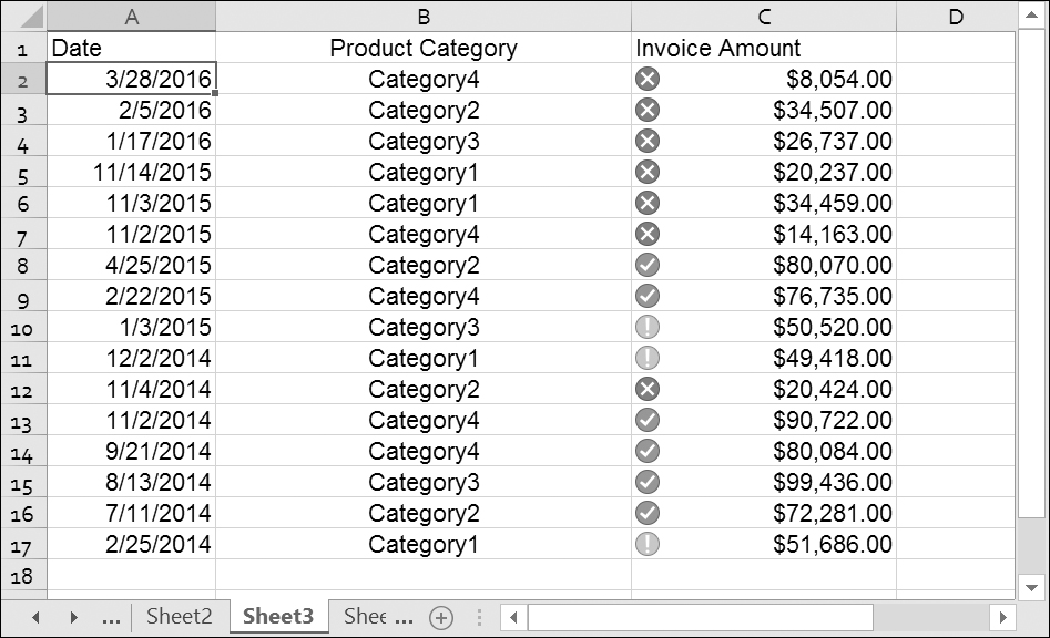
FIGURE 18.12. A column of data with an icon set used in the conditional format.
5. Place the insertion point anywhere inside the code of the IconSetRules procedure and press F8 after each statement to execute the code in step mode.
As mentioned earlier, you can modify the icon set conditions using the dialog box shown in Figure 18.11 or with VBA. Let’s say that instead of using the default percentage distribution with the threshold of >=67, >=33, and <33, you want to use the following criteria: >=80000, >=50000, and <50000.
Let’s take a look at the revised procedure that modifies the formatting rule and applies a filter by cell icon criteria:
Sub IconSetRulesRevised()
Dim iSC As IconSetCondition
Columns("C:C").Select
Selection.SpecialCells(xlCellTypeConstants, 23).Select
With Selection
.FormatConditions.Delete
.AutoFilter
.NumberFormat = "$#,##0.00"
Set iSC = Selection.FormatConditions.AddIconSetCondition
iSC.IconSet = ActiveWorkbook.IconSets(xl3Symbols)
With iSC.IconCriteria(2)
.Type = xlConditionValueNumber
.Value = 50000
.Operator = xlGreaterEqual
End With
With iSC.IconCriteria(3)
.Type = xlConditionValueNumber
.Value = 80000
.Operator = xlGreaterEqual
End With
.AutoFilter Field:=1, Criteria1:=iSC.IconSet.Item(3), Operator:=xlFilterIcon
End With
End Sub
Note that when changing the criteria for the icon set conditional format you do not need to specify the type, value, and operator for IconCriteria(1). This property is read-only. Excel determines on its own the threshold value of IconCriteria(1), and if you try to set it in your code as shown in the example procedure available in online help, you will get a runtime error. The Sort and Filter commands allow you to sort or filter data based on cell icon. The previous procedure demonstrates how you can apply the filter programmatically using an icon in the specified icon set. The results of this procedure are shown in Figure 18.13.
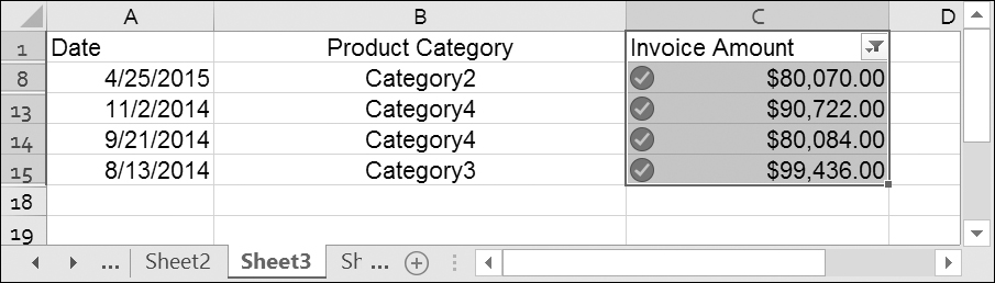
FIGURE 18.13. After running the IconSetRulesRevised procedure, a filter is applied to the Invoice Amount column to display only the cells with invoice values >= 80000.
Let’s say that you only want to highlight cells with values less than 50000. The following procedure creates a formatting rule that produces the output shown in Figure 18.14.

FIGURE 18.14. In this scenario, we use the icon set to draw attention to cells with invoice amounts less than 50000. Notice that by not applying icons to other cells you can easily highlight the problem areas.
Sub IconSetHideIcons()
Dim iSC As IconSetCondition
Columns("C:C").Select
Selection.SpecialCells(xlCellTypeConstants, 23).Select
With Selection
.FormatConditions.Delete
.NumberFormat = "$#,##0.00"
Set iSC = Selection.FormatConditions.AddIconSetCondition
iSC.IconSet = ActiveWorkbook.IconSets(xl3Symbols)
.FormatConditions(1).IconCriteria(1).Icon = xlIconRedCrossSymbol
With iSC.IconCriteria(2)
.Type = xlConditionValueNumber
.Value = 50000
.Operator = xlGreaterEqual
.Icon = xlIconNoCellIcon
End With
With iSC.IconCriteria(3)
.Type = xlConditionValueNumber
.Value = 80000
.Operator = xlGreaterEqual
.Icon = xlIconNoCellIcon
End With
End With
End Sub
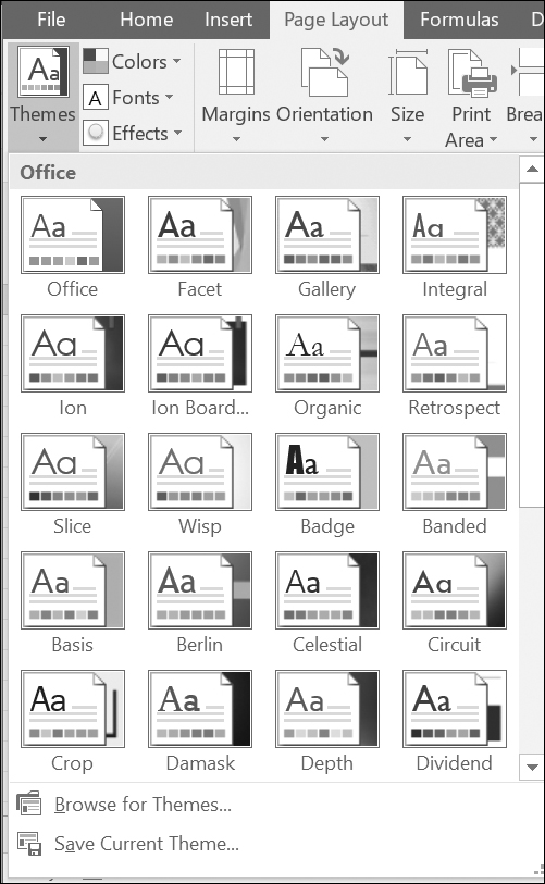
If you need to change the look of the entire workbook, you ought to spend some time familiarizing yourself with document themes. A document theme consists of a predefined set of fonts, colors, and effects, such as lines and fills, that you can apply to the workbook and also share between other Office documents. It is important to note that a theme applies to the entire workbook, not just the active worksheet. There are almost 50 document themes available in the user interface (choose Page Layout | Themes; see Figure 18.15), and you can also create custom themes by mixing and matching different theme elements using the three drop-down controls found in the Themes group on the Page Layout tab (Colors, Fonts, and Effects). Additional themes can also be downloaded from Office Online. When you change the theme, the font and color pickers on the Home tab, and other galleries such as Cell Styles or Table Styles, are automatically updated to reflect the new theme. Therefore, if you are looking to apply a cell background with a particular color, and that color is not listed in the color picker, apply a predefined theme that contains that color, or create your own custom color by choosing the More Colors option in the Font Color drop-down menu.
On the Page Layout tab, the Colors drop-down displays the color groups for each theme and gives you an option to create new theme colors. The Fonts drop-down shows a list of fonts for the theme. Theme fonts contain a heading font and a body text font, which can be changed using the Create New Theme Fonts option in the drop-down. The Effects drop-down displays the line and fill effects for each of the built-in themes and does not give you an option to create your own set of theme effects.
A theme color scheme consists of 12 base colors, as illustrated in Figure 18.16. When applying a color to a cell, the color is selected from the Fill Color drop-down as shown in Figure 18.17.

FIGURE 18.16. The theme colors consist of four text/ background colors, six accent colors, and two hyperlink colors. To display this dialog box, choose Page Layout | Colors | Customize Colors.

FIGURE 18.17. The Fill Color control is used to color the background of selected cells.
On the Home Tab in the Font area of the Ribbon there is a convenient Fill Color button that makes it easy to view the available theme colors (see Figure 18.17). When you click the drop-down arrow next to the Fill Color button, you will see a color palette. The top row in the palette displays 10 base colors in the current color theme (the two hyperlink colors shown in the Create New Theme Colors dialog box are not included). The five rows below show variations of the base color. A color can be lighter or darker. The color name is shown in the tooltip.
If you record a macro while applying the “Blue, Accent 1, Lighter 40%” color to the cell background, you will get the following VBA code:
Sub Macro1()
'
' Macro1 Macro
'
'
Range("F4").Select
With Selection.Interior
.Pattern = xlSolid
.PatternColorIndex = xlAutomatic
.ThemeColor = xlThemeColorAccent1
.TintAndShade = 0.399975585192419
.PatternTintAndShade = 0
End With
End Sub
The pattern properties refer to the cell patterns that can be set via the Format Cells dialog box (Home | Format | Format Cells | Fill). These properties can be ignored if all that’s required is setting the cell background color. The above code can be modified as follows:
Sub Macro1()
'
' Macro1 Macro
'
'
Range("F4").Select
With Selection.Interior
.ThemeColor = xlThemeColorAccent1
.TintAndShade = 0.399975585192419
End With
End Sub
The ThemeColor properties listed in Figure 18.18 specify the theme color to be used.
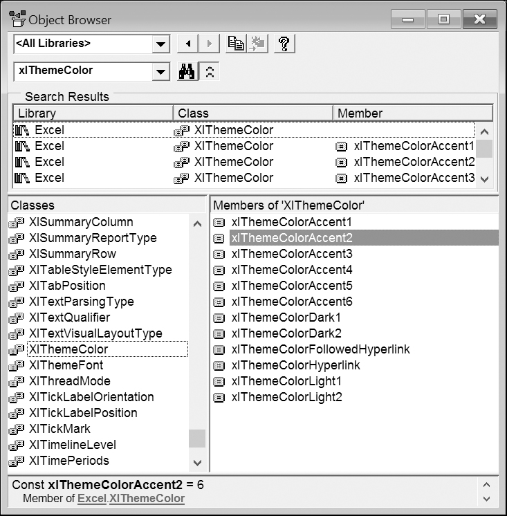
FIGURE 18.18. Theme color constants and values as shown in the Object Browser.
The TintAndShade property is used to modify the selected color. A tint (lightness) and a shade (darkness) is a value from −1 to 1. If you want a pure color, set the TintAndShade property to 0. The value of −1 will result in black, and the value of 1 will produce white. Negative values will produce darker colors, and positive values lighter colors. The TintAndShade value of 0.399975585192419 means a 40% tint (or 40% lighter than the base color). If you change this number to −0.399975585192419, you will get a 40% darker color.
The following procedure loops through the colors in themes 4 through 10 and writes the color index and color variations to the range of cells shown in Figure 18.19.
Sub Themes4Thru10()
Dim tintshade As Variant
Dim heading As Variant
Dim cell As Range
Dim themeC As Integer
Dim r As Integer
Dim c As Integer
Dim i As Integer
heading = Array("ThemeColorIndex", "Neutral", "Lighter 80%", "Lighter 60%", "Lighter 40%", "Darker 25%", "Darker 50%")
tintshade = Array(0, 0.8, 0.6, 0.4, -0.25, -0.5)
i = 0
For Each cell In Range("A1:G1")
cell.Formula = heading(i)
i = i + 1
Next
For r = 2 To 8
themeC = r + 2
For c = 1 To 7
If c = 1 Then
Cells(r, c).Formula = themeC
Else
With Cells(r, c)
With .Interior
.ThemeColor = themeC
.TintAndShade = tintshade(c - 2)
End With
End With
End If
Next c
Next r
ActiveSheet.Columns("A:G").AutoFit
End Sub

FIGURE 18.19. This worksheet was generated by a VBA procedure. When you apply a different document theme, the colors will be replaced by those from the new theme.
The following procedure applies the current theme colors to a range of cells in an active worksheet.
Sub GetThemeColors()
Dim tColorScheme As ThemeColorScheme
Dim colorArray(10) As Variant
Dim i As Long
Dim r As Long
Set tColorScheme = ActiveWorkbook.Theme.ThemeColorScheme
For i = 1 To 10
colorArray(i) = tColorScheme.Colors(i).RGB
ActiveSheet.Cells(i, 1).Value = colorArray(i)
Next i
i = 0
For r = 1 To 10
ActiveSheet.Cells(r, 2).Interior.Color = colorArray(i + 1)
i = i + 1
Next r
End Sub
In the above procedure, the ThemeColorScheme object represents the color scheme of a Microsoft Office theme. In the first For Next loop, the Colors method and the RGB property are used to return a specific color. The color value is then stored in the colorArray array variable and entered in the specified row of the first worksheet column. The second For Next loop applies background color to cells based on the color values stored in the colorArray variable.
The following procedure does more color work in the active sheet, this time using the Interior.ThemeColor property:
Sub ApplyThemeColors()
Dim i As Integer
For i = 1 To 10
ActiveSheet.Cells(i, 3).Interior.ThemeColor = i
ActiveSheet.Cells(i, 4).Value = i
Next i
End Sub
In this procedure, we use the Interior.ThemeColor property to set the background color of cells in the third worksheet column using colors available in the current color scheme. The color scheme value is then written in the corresponding cell in the fourth column. The resulting worksheet (after running the GetThemeColors and ApplyThemeColors procedures) is shown in Figure 18.20.
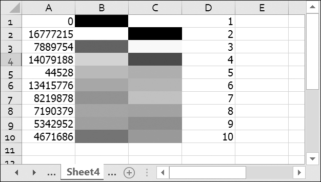
FIGURE 18.20. The background color of the cells was applied with VBA. When you select a different color theme, the background color of these cells (C1:C10) will automatically adjust.
Each new workbook is created with a default theme named Office. The theme information is stored in a separate theme file with the extension .thmx. When you change the theme in the workbook, the workbook’s theme file is automatically updated with the new settings. When you create a custom theme by selecting a new set of fonts, colors, or effects, save the theme in a file so that it can be used in any document in any Office application or shared with other users. You will find your custom theme file in the following location:
\Users\<user name>\AppData\Roaming\Microsoft\Templates\Document Themes
By default the Application Data (AppData) folder is hidden. To access this folder, you will need to modify the folder and search options in Windows Explorer.
To create a test theme named “MyTheme.thmx,” choose Page Layout | Themes | Save Current Theme, change the name to MyTheme.thmx, and press Save.
Now that you’ve created a custom theme, you can apply it programmatically to the workbook using the ApplyTheme method of the Workbook object. Try it out now by entering the following statement on one line in the Immediate window (revise the path as necessary to match the location of the theme file on your computer):
ActiveWorkbook.ApplyTheme "C:\Users\<username>\AppData\Roaming\Microsoft\Templates\Document Themes\MyTheme.thmx"
After you apply a custom theme to a workbook, the theme name should appear in the Custom group of the Themes control, as shown in Figure 18.21.

FIGURE 18.21. After applying a custom theme to a workbook, the theme name appears in the Custom group of the Themes control.
To programmatically load a color theme or font theme from a file, the following VBA statements can be used:
ActiveWorkbook.Theme.ThemeColorScheme.Load ("C:\Program Files (x86)\Microsoft Office\root\Document Themes 16\Theme Colors\Paper.xml")
ActiveWorkbook.Theme.ThemeFontScheme.Load " C:\Program Files (x86)\Microsoft Office\root\Document Themes 16\Theme Fonts\Calibri.xml")
In order to customize some theme components, you need to know how to work with document parts in the Office Open XML file format. You will find information on how to open, read, and modify data in Office XML files in Chapter 28, “Using XML in Excel 2016.”
You can make your worksheets more interesting by adding various types of shapes, such as the cylinder in Figure 18.22. When formatting shapes, you can use document theme colors as shown in the following procedure:

FIGURE 18.22. A Shape object placed on the worksheet uses the theme color scheme.
Sub AddCanShape()
Dim oShape As Shape
Set oShape = ActiveSheet.Shapes.AddShape (msoShapeCan, 54, 0, 54, 110)
With oShape
.Fill.ForeColor.ObjectThemeColor = msoThemeColorAccent4
.Fill.Transparency = 0.5
.Line.Visible = msoFalse
End With
Set oShape = Nothing
End Sub
In the above procedure, we declare an object variable of type Shape and then use the AddShape method of the ActiveSheet Shapes collection to add a new Shape object. This method has five required arguments. The first one specifies the type of the Shape object that you want to create. This can be one of the constants in the msoAutoShapeType enumeration (check out the online help). Excel offers a large number of shapes. The next two arguments tell Excel how far the object should be placed from the left and top corners of the worksheet. The last two arguments specify the width and height of the shape (in points). To specify the theme color of the Shape object, set the ObjectThemeColor property of the ColorFormat object to the required theme. To return the ColorFormat object, you must use the ForeColor property of the FillFormat object. The FillFormat object is returned by the Fill property of the Shape object:
oShape.Fill.ForeColor.ObjectThemeColor = msoThemeColorAccent4
Next, set the degree of transparency to make sure that the shape does not obstruct the data. The last line removes the border from the shape.
The previous procedure places a Shape object over the data in column B.
The following procedure can be run to programmatically remove shapes from the worksheet:
Sub RemoveShapes()
Dim oShape As Shape
Dim strShapeName As String
With ActiveSheet
For Each oShape In .Shapes
strShapeName = oShape.Name
oShape.Delete
Debug.Print "The Shape Object named " & strShapeName & " was deleted."
Next oShape
End With
End Sub

|
Working with Shapes in VBA |
|
While you can look up the properties and methods of the Shape object in the online help, don’t forget Excel’s most useful tool—the macro recorder. Use Shape object recording to get a quick start in writing VBA code that inserts, positions, formats, and deletes shapes. |
Sparklines are tiny charts that can be inserted into a single cell to highlight important data trends and increase readers’ comprehension.
There are three types of sparklines in Excel: Line, Column, and Win/Loss. They can be inserted via the corresponding button in the Sparklines group on the Ribbon’s Insert tab (Figure 18.23).

FIGURE 18.23. The Sparkline group on the Insert tab offers three buttons for inserting tiny charts into a cell.
To manually insert a sparkline graphic, click in the cell where you want the sparkline to appear and choose Insert. In the Sparklines group, click the type of sparkline you want to insert. At this point, Excel will pop up the Create Sparklines dialog box (Figure 18.24) where you can choose or enter the data range you want to include as the data source for the sparklines and the location range where you want them to be placed.

FIGURE 18.24. Selecting the location and data range for sparklines.
In Figure 18.24, we’d like to compare the performance of users during each quarter of fiscal year 2015. After making selections in the Create Sparklines dialog box and clicking OK, Excel activates the Sparkline Tools–Design context tab, where you can format the sparkline by showing points and markers, changing sparkline or marker colors, switching between the types of sparklines, and more. Figure 18.25 displays the final result of inserting and applying data point formatting to the sparklines.

FIGURE 18.25. Sparklines in column G make it easy to spot the trends in users’ performance.
|
Handling Hidden Data and Empty Cells by Sparklines |
|
If you hide rows or columns that are used in a sparkline, the hidden data will not appear in the sparkline. You can specify how empty cells should be handled in the Hidden and Empty Cells Settings dialog box (choose Sparkline Tools | Design | Sparkline | Edit Data | Hidden and Empty Cells). |
Sparklines are dynamic. They will automatically adjust whenever the data in the cells they are based on changes. Sparklines can be copied, cut, and pasted just like formulas. For bigger or wider sparklines, simply increase the width of the row or column. To get rid of the sparklines, use the Clear option in the Design context menu, and select Clear Selected Sparklines or Clear Selected Sparkline Groups.
Because a sparkline is a part of a cell’s background, you can display text or formulas in cells containing sparklines, as shown in Figure 18.26.
|
Sparklines and Backward Compatibility |
|
When you open a workbook containing sparklines in older versions of Excel (2007/2003), you will see blank cells. When you edit a file with sparklines in Excel 2007 the sparklines will not be visible, but they will appear again if the file is loaded in more recent versions of Excel, provided that the cells with sparklines were not deleted. |
In Figure 18.24 we created multiple sparklines at once by choosing one data range (B2:E6). This caused the sparklines to be automatically grouped. When you click a grouped sparkline, you should see a thin blue line around the group. Each sparkline group contains the same formatting settings. You can format each sparkline separately by breaking the group. Simply select the sparkline you want to format differently, and choose Sparkline Tools | Design | Group and click Ungroup. The selected cell will be ungrouped from the group. Now you can format that sparkline as desired without affecting other sparklines. For example, in Figure 18.27 the sparkline in Row 4 was ungrouped and the type of sparkline was then changed to column type. To break the entire group, select all the cells containing sparklines and click Ungroup.

FIGURE 18.27. Ungrouping sparklines lets you format them independently of other sparklines.
The Excel object model contains objects, properties, and methods that allow developers to use VBA to create and modify sparklines in their worksheets. To get an idea of how sparklines fit into the object model, take a look at Figure 18.28.

FIGURE 18.28. Choose the Object Browser from the VBE View menu (or press F2) to quickly locate objects, methods, and properties that can be used to program sparklines with VBA. Next, select the name of the object, property, or method that interests you, and click the question mark button at the top of the Object Browser to pop up the help topic.
Each sparkline is represented by a Sparkline object, which is a member of a SparklineGroup object. A SparklineGroup object can contain one or more Sparkline objects. You can have multiple SparklineGroup objects (collections of sparkline groups) in a worksheet. The Range object’s SparklineGroup property returns a SparklineGroups object that represents an existing group of sparklines from the specified range.
Hands-On 18.2 demonstrates how to use VBA to read the information about sparklines contained in a worksheet.
1. Working with the C:\VBAExcel2016_ByExample\Chap18_VBAExcel2016.xlsm workbook, switch to the Visual Basic Editor screen and insert a new module into VBAProject (Chap18_VBAExcel2016.xlsm).
2. In the module’s Code window, enter the following GetSparklineInfo procedure:
Sub GetSparklineInfo()
Dim spGrp As SparklineGroup
Dim spCount As Long
Dim i As Long
spCount = Cells.SparklineGroups.count
If spCount <> 0 Then
For i = 1 To spCount
Set spGrp = Cells.SparklineGroups(i)
Debug.Print "Sparkline Group:" & i
Select Case spGrp.Type
Case 1
Debug.Print "Type:Line"
Case 2
Debug.Print "Type:Column"
Case 3
Debug.Print "Type:Win/Loss"
End Select
Debug.Print "Location:" & spGrp.Location.Address
Debug.Print "Data Source: " & spGrp.SourceData
Next i
Else
MsgBox "There are no sparklines in the active sheet."
End If
End Sub
3. Activate the worksheet that contains sparklines and run the above procedure. Assuming you ran the procedure while the sheet displayed in Figure 18.27 was active, the following information was retrieved into the Immediate window.
Sparkline Group:1
Type:Column
Location:$G$4
Data Source: B4:E4
Sparkline Group:2
Type:Line
Location:$G$2,$G$3,$G$5,$G$6
Data Source: B2:E2,B3:E3,B5:E5,B6:E6
The next Hands-On shows how you can create a sparkline Win/Loss report from scratch using VBA. The Win/Loss sparkline bar chart type is used to display Profit versus Loss or Positive versus Negative comparison.
1. In the C:\VBAExcel2016_ByExample\Chap18_VBAExcel2016.xlsm workbook, switch to the Visual Basic Editor screen and add the following procedures just below the GetSparklineInfo procedure that you created in the previous Hands-On:
Sub CreateSparklineReport()
Dim spGrp As SparklineGroup
Dim sht As Worksheet
Dim cell As Range
Dim spLocation As Range
Workbooks.Add
Set sht = ActiveSheet
EnterData sht, 3, "Month", "Sales Quota", "Sales $", "Difference"
EnterData sht, 4, "January", "234000", "250000", "=C4-B4"
EnterData sht, 5, "February", "211000", "180000", "=C5-B5"
EnterData sht, 6, "March", "304000", "370000", "=C6-B6"
Range("B4:D6").Style = "Currency"
Columns("A:D").AutoFit
Range("A1").Value = "Win/Loss"
Set spLocation = sht.Range("B1")
Set spGrp = spLocation.SparklineGroups.Add(xlSparkColumnStacked100, "D4:D6")
spGrp.SeriesColor.ThemeColor = 2
spLocation.SparklineGroups.Item(1).Axes.Horizontal.Axis.Visible = True
End Sub
Sub EnterData(sht As Worksheet, rowNum As Integer, ParamArray myValues() As Variant)
Dim j As Integer
Dim count As Integer
count = UBound(myValues()) + 1
j = 1
For j = j To count
sht.Range(Cells(rowNum, 1), Cells(rowNum, count)) = myValues()
Next
End Sub
2. Run the CreateSparklineReport procedure.
After running the procedure you should see the Win/Loss report in a new workbook as depicted in Figure 18.29.
In Figure 18.29, the Win/Loss sparkline in cell B1 compares sales data during the first three months of the year with the sales quota for each month. The source range for the sparkline is located in column D, which contains the difference between monthly sales and the monthly quota. A quick glance at cell B1 reveals that the sales quota was not met in February.
Most people use the Format Painter tool on the Ribbon’s Home tab (the paintbrush icon) to quickly copy formatting to other cells of the same worksheet or from one worksheet to another. However, when you create complex worksheets with different types of formatting, it is a good idea to save all your formatting settings in a file so you can reuse them whenever you need them. This can be done via the Styles feature. Cell styles can contain format options such as Number, Alignment, Font, Border, Fill, and Protection. If you change the style after you have applied it to your worksheet, Excel will automatically update the cells that have been formatted using that style. Styles are easier to find and apply, thanks to the existence of galleries like those illustrated in Figure 18.30. To apply a style to a cell, simply select the cells you want to format with the style, and click on the appropriate style in the gallery (available by clicking Cell Styles). Styles are based on the current theme. You can also apply them to Excel tables, PivotTables, charts, and shapes. Excel offers a large number of built-in styles. You can modify, duplicate, or delete the existing styles and add your own—simply right-click the style in the gallery and select the option you need.
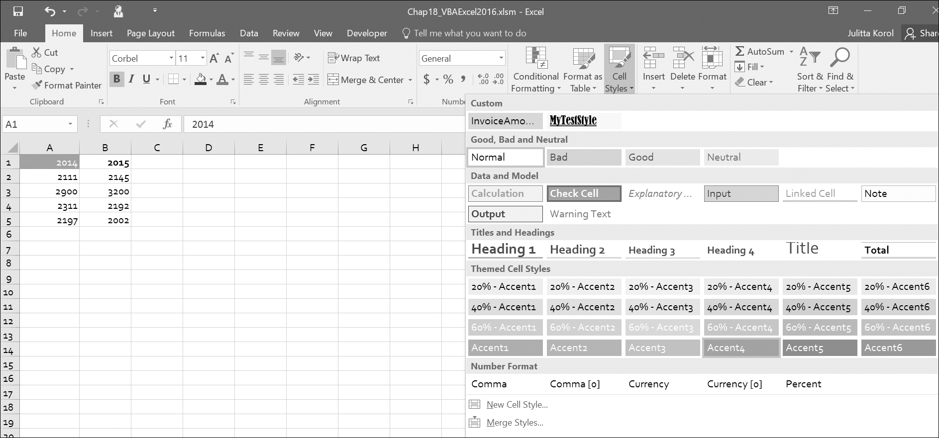
FIGURE 18.30. You can see the preview of how the style will look before you apply the style. If the built-in style does not suit your needs, you can create your own custom style.
To find out the number of styles in the active workbook, use the following statement:
MsgBox "Number of styles=" & ActiveWorkbook.Styles.Count
Excel tells us that there are 49 styles defined for a 2016 workbook. Use the Styles collection and the Style object to control the styles in a workbook. To get a list of style names, let’s iterate through the Styles collection:
Sub GetStyleNames()
Dim i As Integer
For i = 1 To ActiveWorkbook.Styles.Count
Debug.Print "Style " & i & ":" & ActiveWorkbook.Styles(i).Name
Next i
End Sub
The above procedure prints the names of all workbook styles into the Immediate window. The style names are listed alphabetically.
To add a style, use the Add method, as shown in the following example procedure:
Sub AddAStyle()
Dim newStyleName As String
Dim curStyle As Variant
Dim i As Integer
newStyleName = "SimpleFormat"
i = 0
For Each curStyle In ActiveWorkbook.Styles
i = i + 1
If curStyle.Name = newStyleName Then
MsgBox "This style " & "(" & newStyleName & ") already exists. " & Chr(13) & "It’s the " & i & " style in the Styles collection."
Exit Sub
End If
Next
With ActiveWorkbook.Styles.Add(newStyleName)
.Font.Name = "Arial Narrow"
.Font.Size = "12"
.Borders.LineStyle = xlThin
.NumberFormat = "$#,##0_);[Red]($#,##0)"
.IncludeAlignment = False
End With
End Sub
The above procedure adds a specified style to the workbook’s Styles collection provided that the style name is unique. The procedure begins by checking whether the style name has already been defined. If the workbook has a style with the specified name, the procedure ends after displaying a message to the user. If the style name does not exist, then the procedure creates the style with the specified formatting. Notice that if you do not wish to include a specific formatting feature in the style, you can set the following properties to False: IncludeAlignment, IncludeFont, IncludeBorder, IncludeNumber, IncludePatterns, and IncludeProtection. For example, a setting of False omits the HorizontalAlignment, VerticalAlignment, WrapText, and Orientation properties in the style. The default setting for these properties is True.
The custom style is added to the Styles collection. To find out the index number of the newly added style, simply rerun this procedure.
To programmatically apply your custom style to a selected range, run the following code in the Immediate window:
Selection.Style = "SimpleFormat"
To check out the settings the specific style includes, select the formatted range of cells and choose Home | Cell Styles to display the gallery of styles. Right-click the name of the selected style and choose Modify. Excel displays the dialog box shown in Figure 18.31.

FIGURE 18.31. This dialog box displays the formatting settings of the SimpleFormat style that was created earlier by a VBA procedure.
The following code removes formatting applied to the selected range:
Selection.ClearFormats
The previous statement returns selection formats to the original state, but does not remove the style from the Styles collection. To delete a style from a workbook, use the following statement:
ActiveWorkbook.Styles("SimpleFormat").Delete
If you have already applied formats to a cell, you can create a new style based on the active cell:
Sub AddSelectionStyle()
Dim newStyleName As String
newStyleName = "InvoiceAmount"
ActiveWorkbook.Styles.Add Name:=newStyleName, BasedOn:=ActiveCell
End Sub
By default Excel creates a new style based on the Normal style. However, if you have already applied formatting to a specific cell and would like to save the settings in a style, use the optional BasedOn argument of the Styles collection Add method to specify a cell on which to base the new style.
The custom styles you create can be reused in other workbooks. To do this you need to copy the style information from one workbook to another. In VBA, this can be done by using the Merge method of the Workbook object Styles collection:
ActiveWorkbook.Styles.Merge " Report2016.xlsx"
Assuming that you have defined some cool styles in the Report2016.xlsx workbook, the above statement copies the styles found in the specified workbook to the active workbook.
In this chapter, you learned how to use VBA to apply basic formatting features to your worksheets to make your data easier to read and interpret. You also learned advanced formatting features such as conditional formatting and the utilization of tools such as data bars, icon sets, color scales, shapes, and sparklines, as well as themes and cell styles.
The next chapter focuses on the customization of the Ribbon interface and context menus in Excel.