Chapter 9
Synthetics

In earlier chapters, the discussion was put forth showing how investors use options to manage the volatility of individual positions or a portfolio of positions. These are powerful techniques investors can use to obtain their investment objectives while managing downside risk. The other broad category of uses for options is the creation of synthetic positions. A synthetic is simply a derivative contract or combination of contracts, which replicates the return performance of a particular asset, security, or market index. Options enable the creation of synthetic positions because there is a deterministic relationship between puts, calls, and the underlying instrument. This relationship, by definition, must be arbitrage free, as a violation of this condition would allow investors to combine positions in the underlying asset along with their associated options in a way that would guarantee a riskless profit. The relationship between the security and its associated options is defined by put–call parity, which is discussed in detail below.

Put–Call Parity

Put–call parity defines the relationship between the prices of a European call, a European put, the underlying security, and the risk-free asset. For this relationship to hold, the strike price and the time to expiration of the put and the call must be identical. In addition, the risk-free asset that is typically defined as a U.S. Treasury bill must have the same maturity date as the expiration date of the two options. In the case of equity securities, the equation for put–call parity is defined below. Put–call parity does not just apply to stocks and their related options. It governs the relationship between the price of any asset and its associated options.

The intuition behind this equation should be very clear. The left-hand side of the equation describes a stock with a married put having the same payoff pattern as holding cash plus a call option. Given this identity, if the price of the stock rises by the expiration date of the put, the investor can sell the stock for a gain while the put expires worthless. If the price of the stock falls below the strike price of the put option, the investor can exercise her right and sell the stock to the put writer at the agreed upon strike price. This will minimize investor loss, which is equal to the starting stock price less the option's strike price less the premium paid on the put option.

The right-hand side of the equation is another way of describing the same payoff pattern. Instead of buying stock and a married put, the investor buys a call option, keeping the rest of her assets in credit and interest rate risk-free cash equivalents. If the price of the underlying stock is above the strike price by expiration, the investor exercises the call and sells the stock purchased for a gain. If, on the other hand, the price of the stock falls, the call expires worthless, leaving the investor with cash. All that is lost in this scenario is the option premium on the call.

The beauty of put–call parity lies in its simplicity, requirement for minimal assumptions, and ease of implementation. Put–call parity allows for the static replication of any of its four elements. In addition, with the assumption that traders can freely borrow and lend at the same rate, cash on hand is not necessary to structure a trade. In theory, borrowing funds for the term of the options can finance the underlying asset and the relationships still holds. Furthermore, it does not require the existence of a forward contract, although one can be created synthetically. In addition, put–call parity presents the relationship of static replication. In a static replication, the reference asset and the replicating portfolio have the same cash flows. By contrast, dynamic replication does not have the same cash flows as the reference asset. A good example of dynamic replicating is gamma scalping. The payoff pattern of a call option is created dynamically by purchasing the underlying asset as its price rises and selling it as its price falls. The end result is a payoff pattern that looks identical to the final payoff pattern of a call option, but the cash flows are different.

One way to think about the right-hand side of the equation is that it is akin to a cash-covered call. To ensure that the buyer of the call can pay for the stock in the event the call is exercised, the buyer must hold enough cash to purchase the stock. Therefore, the quantity of the risk-free asset the seller must hold is equal to the present value of the strike price of the call option.

In this relationship, K represents the strike price of the options, r is the interest rate on the risk-free asset, and t is the time to expiration of the put and call options, which must be the same as the maturity date of the Treasury bill. The implication of put–call parity is quite profound. It tells us that there is equivalence between puts and calls even though they have very different payoff patterns. As a result, we can replicate any delta-neutral portfolio. If a call has a delta of D, for example, then buying a call and selling D number of shares of stock is equivalent to selling a put and buying shares of stock. This is a very important relationship and market makers use it regularly to manage the price risk of their inventory.

Synthetically Replicating Stock

By rearranging the equation of put–call parity above, we can see that we can replicate the return characteristics of stock by purchasing a call, selling a put with the same strike price and time to expiration, while holding the appropriate amount of cash.

Since the relationship between the four elements that make up put–call parity exists in an arbitrage-free environment, the advantage of holding synthetic stock versus real stock is not entirely obvious. There are times, however, where it is cheaper to buy stocks synthetically than buying the security outright. One example is the situation where there is heavy short interest on a stock, and as a result it is expensive to borrow. Since market makers borrow stock and sell it short against their long call positions, they must pay the stock lender a fee to do so. This affects the price of a call by driving down its price. Since the market makers must pay a fee to hedge their call position, the call is worth less to them. By the same token, if a market maker buys put options, they purchase stock as a hedge. Now that they own stock, they can take advantage of the high cost of borrowing by lending the stock to short sellers, who have to pay them a fee. Since they can make a return on their stock holdings, the puts have more value to them. As a result, they can pay a higher price for puts. In short, a trader can buy cheap calls and sell expensive puts while holding cash, and in doing so, own synthetic stock at a lower price than the quoted price of the shares in the marketplace.

To see how much we could improve returns by synthetically creating stock versus purchasing stock outright, it's useful to walk through a numerical example. To do this, we will continue with the example presented in Chapter 8, where we walked through the mathematics of computing the implied borrowing cost extracted from option prices. All the factors of those numerical examples are the same, and we will assume there is a 12 percent borrowing cost to the underlying stock. In making this assumption, we get the following results:

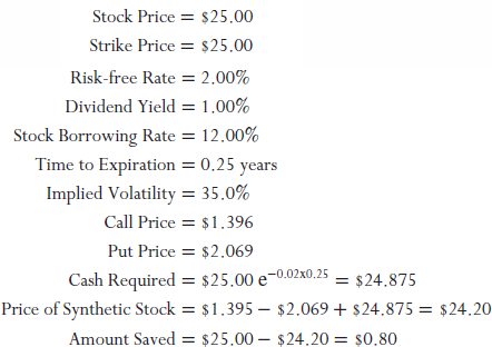
This analysis shows that the cost of creating stock synthetically is $24.20. This is a 3.2 percent discount to the price of the underlying stock. This is a direct savings to an investor who might want to own the stock, but chooses to buy it synthetically instead of buying it outright. The reason why this apparent arbitrage exists is due to industry structure. Individual investors do not have the opportunity to lend their stock holdings and collect a fee. Most people are under the impression that brokerage firms only make money by the commissions they charge their customers to transact securities. But brokerage firms have other very important sources of revenue that cover their cost of doing business. One is lending money to investors who buy securities on margin. The second is through securities lending. When an investor buys a security, the brokerage firm holds that security in their name. When a short seller needs a stock, she must borrow it first and then sell it into the marketplace. The lender of stock wants to be sure that it eventually bets the stock back. For protection against a default on the stock loan, the broker-dealer demands cash in an amount equal to the value of the stock lent out. The broker-dealer invests that cash in short-term securities to earn a return. Most stocks are not hard or expensive to borrow. Under these circumstances, the only revenue the broker-dealer earns is interest on the cash collateral. But there are situations where there is a high demand to borrow a stock and the broker-dealer can charge stock borrowers a premium to do so. When they do, this creates an additional revenue source for the broker-dealer. Broker-dealers, however, do not share this revenue with their retail clients. This is not the case for institutional clients, such as corporate pension plans. Firms performing securities safekeeping for these large institutions have programs where they share the revenue generated from securities lending with the owners of the securities. For these folks, there is a far smaller advantage of owning synthetics versus the actual securities as they get a portion of the securities' lending revenue. Since retail investors do not capture the returns provided by securities lending, they can greatly benefit by using synthetics.

Synthetically Replicating a Call

Not only can an investor replicate stock with a combination of puts, calls, and cash, but put–call parity allows the investor to create a call synthetically as well. By rearranging the standard equation of put–call parity, we can replicate a call by purchasing stock, buying a put, and financing those positions by borrowing the present value of the strike price of the underlying options.

Just as investors can arbitrage the difference between a synthetic stock and a reference stock, investors can arbitrage the price difference between the call and the synthetic call. In the previous example, the opportunity to do so might occur when a stock is expensive to borrow or when there is a dislocation in price due to a large buyer or seller of a particular option with a specific time to expiration and strike price. Continuing with the example, the following shows the price of a call option with one created synthetically:

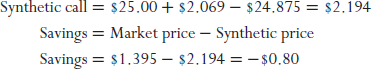
The comparison shows there is an $0.80 cost advantage of buying a call in the market versus creating one synthetically. We might be tempted to believe there is an arbitrage opportunity to be had by selling a synthetic call for $2.194 and buying a real one for $1.395. This would leave us with $0.80 in our pocket. But this apparent arbitrage is just an illusion. The exercise of creating synthetic stock shows us that the cost of borrowing was worth $0.80 a share. So if we bought the option and sold a synthetic one, the $0.80 up-front advantage would be eaten up by the cost of borrowing stock when creating the synthetic call. So a long real/short synthetic pair trade would only earn a profit if the borrowing rate fell during the life of the trade. This would reduce the cost of carrying the synthetic call and increase the price of the real call. This, however, is a far more difficult arbitrage for the individual investor to capture. This is true for two reasons. The first impediment to capturing this arbitrage is that individual investors cannot borrow at the risk-free rate. They have to pay the broker loan rate to borrow cash, which typically runs 6 percent or more in today's market. To figure out the breakeven broker loan rate, we need to determine the point where higher cash borrowing costs offset the stock borrowing. This is done by setting the synthetic call price equal to the quoted call price in solving for the cost of carry.

Synthetically Replicating a Put

Just as a stock or call option can be created synthetically, a put option can also be created synthetically as well. This is done by purchasing a call, selling a stock short, and holding the present value of the option's strike price in a credit and market risk-free cash equivalent security. We can see this by rearranging the equation of put–call parity solving for the value of a put:

By continuing with our example, we see that the value of a synthetic put is equal to $1.27. By selling a put option available in the marketplace and purchasing an equivalent put synthetically, we will capture $0.94 advantage:

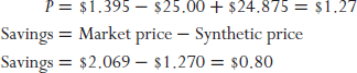
This comparison shows that there is a $0.80 cost advantage of buying a synthetic put, versus one trading on an exchange. Once again, we might be tempted to believe there is an arbitrage opportunity to be had by purchasing a synthetic put for $1.27 and selling a real one for $2.069. This would also leave the investor with $0.80 in his pocket. Like the case of a synthetic call, this apparent arbitrage is just an illusion, and it goes back to the discount on creating synthetic stock. The process of creating a synthetic put entails shorting stock. The cost of borrowing that stock will consume the $0.80 advantage over the life of the trade. So a long synthetic/short real pair trade would only earn a profit if the borrowing rate fell during the life of the trade. This would increase the value of the synthetic put and decrease the price of the real put. In the end, like the situation of a pairing a real and synthetic call, this is really just a method for trading the borrowing rate.

Synthetically Replicating Cash

Since put–call parity governs the relationship between the underlying security, its options, and cash, we can use the relationship to synthetically borrow or lend cash. This is a tactic that is used by institutions from time to time to generate liquidity and/or invest in a high-yielding synthetic asset whose return is driven, at least in part, by the cost of borrowing. To create an investable asset, someone buys stock, sells a call, and buys a put to hedge it. We can see this by rearranging the equation of put–call parity solving for cash. Within the framework of put–call parity, the cash required to buy stock purchased is perfectly hedged with an option structure that has a delta of −1.0. The long stock and option structure leaves the investor with a position that is perfectly hedged.

To generate cash, we do just the opposite. The appropriate structure is to sell stock, buy a call, and sell a put. In this example, this structure would generate $25.675 in cash up front and would earn an additional $0.129 by investing the proceeds in the risk-free asset at 2 percent a year for three months.

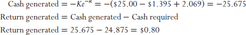
There is no real advantage for pursuing this approach, as it is a yield strategy. Yield strategies depend on the passage of time to collect income. In this case, the investor would collect $25.675 up front, invest that sum to earn interest, but give it all back in the borrowing cost of the stock sold short. While this is not a viable strategy for the individual investor, it might be available for a broker-dealer whose customers might own the underlying stock. Under these circumstances, the broker-dealer can borrow the customer stock at no cost and implement the strategy, capturing the $0.80 advantage per share of stock. Furthermore, a broker-dealer could use this as a cheap source of funding to cover the cash needed to pay for other positions in their trading book.

In this section we discussed the traditional ways option professionals create options and securities synthetically. We show that when there is a heavy cost of borrowing in the underlying security, individual investors can take advantage of this circumstance by creating the asset synthetically. In doing so, they can capture the implied lending income reflected by the discount available from the synthetic security. The beauty of this strategy is that investors do not have to lend their securities, so anyone can take advantage of the opportunity. Furthermore, the synthetic security will automatically be converted to a real one at expiration. If the price of the underlying is above the strike, the investors exercise their call and take delivery of the stock. Alternatively, if the price of the underlying stock is below the strike price of the two options, stock will be put to them. Either way, the investors now own stock. If the cost of borrowing remains at expiration, the trade can be rolled and repeated over until such time that the implied borrowing rate ceases to exist.

Synthetics go beyond simply replicating stock with puts, calls, and cash, or any of the other permutations suggested by put–call parity. Corporate finance theory tells us there is a relationship between the values of the firm's assets and the claims on those assets. The primary claims on corporate assets are debt and equity securities. In the following section, we will present a discussion about how we might synthetically create corporate debt securities by using options on the company's equity securities.

Creating Corporate Debt Synthetically

Corporations raise both debt and equity capital to fund their operations. The equity capital in private firms comes from their owner/operators, other individual investors and/or institutional investors such as private equity firms and venture capitalists. Public companies raise their equity in the capital markets. Capital market investors are individuals who purchase stock directly or indirectly through mutual funds and their retirement plans. Institutional investors, such as insurance companies, pension funds, and hedge funds participate in these markets as well. Insurance companies for example, purchase stocks and bond in public companies with the insurance premiums they collect from their customers. These funds are invested with the intention of earning a return until the day comes when the insurance company needs to make good on its promises.

The capital structure of most companies' equities tends to be quite simple, as a good number of companies only issue common stock. Some companies such as banks and utilities also issue preferred stock, as they have a shareholder base that looks to dividends for their cash-flow needs. Most companies borrow money to fund their operations in addition to sourcing equity capital. That tends to be a more complex aspect of the firm's capital structure. It is not uncommon for firms to borrow money from a bank collateralized by receivables, inventory, real estate, and/or equipment. At the same time, they might borrow money from an insurance company or the capital markets on an unsecured basis. Since unsecured lenders get paid in bankruptcy only after the secured lenders are paid, these loans are more risky and companies have to pay a higher rate of interest to compensate investors for that risk.

Some firms look for more esoteric ways of raising capital that meets their funding and cash flow needs. These firms might issue “quasi-equity” securities in the form of convertible bonds, which allow the investors to convert their loan into the equity of the issuing firm at their discretion. Companies like to issue these securities, as the conversion feature of the imbedded call option has value. By selling an imbedded call, which has value, it allows the issuing company to offer these securities at a lower rate of interest. Investors like convertible securities because it allows them to earn equity rates of return should the company do extremely well. At the same time, it provides some cash flow while they wait. Furthermore, they get the added benefit of owning a security that resides higher in the capital structure relative to equity, giving the convertible securities investor some downside protection in a bear market or bankruptcy scenario. Some companies are tight on cash flow in the short to intermediate term because they are making large investments in plant and equipment, for example. These companies often issue pay in kind (PIK) bonds. Issuers of PIK bonds have an option of sorts. PIK bonds give the issuer the flexibility of paying interest with additional bonds instead of cash. Highly levered capital-intensive firms often issue this type of bond. These firms value the flexibility to issue additional bonds to conserve cash in the short run and to match their operating cash flow with their debt service requirements.

Companies issue debt securities when they want to expand their businesses, buy back stock, or pay off other existing debts. When firms issue additional equity, they increase the balance of the existing equity securities outstanding. When firms issue debt they usually create a new security in the company's capital structure, as the terms of the new issue are usually different from older outstanding issues. Over time, firms may issue a large number of different tranches of debt, making each issue somewhat illiquid. Some tranches may not be particularly large. More often than not, small debt issues are “put away” by institutional investors who plan to hold them to maturity. These factors serve to limit liquidity in the debt issues of many companies. Investors who might want to buy those outstanding issues may not be able to find sellers or may not be able to find securities in sufficient size to satisfy their needs. As result, these investors must find debt securities issued by other companies that meet their investment objective and risk profile. The alternative that few investors pursue is to create debt securities synthetically. It is possible to create debt securities synthetically because there is a relationship between the value of a firm and the value of the financial claims on that firm's assets.

Depending on the operational risk of a business and/or the risk tolerance of investors and managers, companies will pursue different capital structures. High-risk companies, such as development-stage biotech companies, often finance themselves entirely with equity. Companies that are somewhat less risky, such as mature technology companies, often finance themselves with modest amounts of debt. Companies borrow as an alternative to issuing equity as a means of creating financial leverage designed to increase returns to shareholders. Since interest payments are tax deductible for a company, financial leverage lowers a company's income tax liability as well. This tax shield has value to shareholders by increasing after-tax cash flow. Companies with low business risk, such as regulated utilities, produce steady cash flow. With steady cash flow and hard assets to pledge as collateral, debt service is more assured. As a result, electric utilities are often financed with high levels of debt. Other times, investors and managers finance manufacturing companies with high levels of debt to retain ownership, while minimizing their equity contribution at risk. High levels of debt are used simply for the purpose of maintaining control of the enterprise.

When a company is capitalized purely with equity, all the asset price performance risk is born by shareholders. Under these circumstances, asset risk and equity risk are identical. When some portion of the company is capitalized with debt, some of the asset price risk is shifted to the lenders. If debt levels are low, the asset price risk transferred to the lenders is quite small. This is the situation common to investment-grade corporate bonds. These loans are relatively safe and pay a low yield premium relative to U.S. Treasury securities, which are thought of as credit risk-free. If the debt levels are high, the asset price risk shifted to the lenders is relatively high. This is the situation common to high-yield bonds, often referred to “below-investment grade” or junk bonds. Having more risk, these corporate obligations pay a higher rate of interest vis-à-vis investment-grade corporate bonds. At the end of the day, the yield premium companies must pay over a U.S. Treasury note to issue debt securities is a reflection of how much asset risk has been transferred to lenders. At the end of the day, asset risk does not change by the way a company is capitalized. It only changes how much risk each claim holder must carry (see Exhibit 9.1).

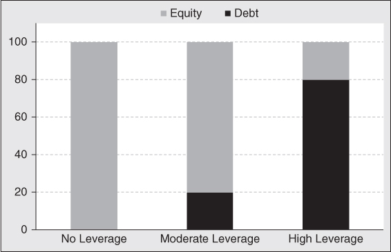
Exhibit 9.1 Capital Structure Examples

Option-pricing theory allows us to think about a company's equity as a call option on the value of a company's assets. If the value of a firm's assets exceeds the value of its liabilities, equity investors can exercise their option to buy the company's assets. Upon exercise, the investor can sell the company's assets, repay the debt, and keep the residual. If the value of the company's assets falls below the face value of its liabilities, the equity investor lets the firm go into liquidation. This is akin to allowing their call option to expire worthless. The lenders now have control of the assets, which they sell as repayment for some or all of the company's debt. Notice that when shareholders let their call options expire, this is equivalent to “putting” the company's assets to the lenders. Thought of in this way, we can think of lenders as put sellers on the value of a company's assets. The strike price of that put is equal to the face value of the company's debt. The time to expiration on that put is equal to the tenor of the debt security issued. Since the company can file bankruptcy at any time, that put the lenders sell is an American-style option.

In a default scenario, it is very rare that the value of a company's assets will fall to zero. Secured lenders have first claim on the assets pledged against the loan. Unsecured lenders capture value that is left over after the secured lenders are made whole. Take, for example, a company that has two loans outstanding. One loan is secured by the company's manufacturing plant. The second loan is unsecured. When the company is liquidated in a bankruptcy proceeding, the funds received by selling the facility are used to repay the secured lender. If there is something left over, that value will accrue to the unsecured lenders. As a result, even unsecured lenders are likely to recover some value when a company defaults on its debt. Naturally, secured lenders will recover more than unsecured lenders since they have first claim on company assets. Since lenders have effectively sold a put on the company's assets to the shareholders, we can recreate the investment performance of debt securities by selling a put option on the company's assets with a strike price equal to the face value of the company's debt, and a time to expiration equal to the tenor of the loan. At the same time, lenders effectively own a put on the company assets, as they have the right to sell those assets they take control of in a bankruptcy proceeding. The strike price of this option is equal to the expected value of the company's assets in a bankruptcy scenario. The strike price of this put is equal to the value of the company's assets in a quick, distressed liquidation. In essence, lenders are not really short a naked put. They are short a put spread with the upper strike equal to the loan amount and the lower strike equal to the corporation's expected liquidation value which is the same as the amount the lender expects to recover on a defaulted loan.

Credit rating agencies such as Moody's and Standard & Poor's have done historical studies of corporate and sovereign defaults. With this data, they are able to estimate default rates by credit rating and loan recovery rates parsed by industry and where the loan resides in a company's capital structure. Since these are the result of real-life situations, they also provide a good foundation for estimating the strike price of the recovery option.

Putting these two elements together, we can synthesize the return performance of a corporate loan by selling a put with a strike price equal to the face value of a company's debt and buying a put with the strike price equal to the expected recovery amount on a defaulted loan. The return on this short put spread captures the effects of a change in company assets on the value of corporate debt. It does not capture the returns driven by credit risk-free rates. To capture those returns, we must buy a credit risk-free instrument, a U.S. Treasury bond with a maturing date equal to the maturity of the corporate bond being replicated.

These equations describe the conceptual formulation for understanding the behavior of credit-risky corporate debt. Creating a short put spread on a company's assets is problematic, as markets for options on company assets do not exist. Fortunately, there are liquid markets for options on a public company's equity securities. Since the value of a company's equity is directly related to the value of its assets, equity options are a less than perfect but usable instrument to replicate the performance of options on assets. To build an understanding of how this process works, it is useful to walk through an example.

Assume, we want to replicate a five-year unsecured corporate bond that is currently priced at $94.00 paying an annual coupon of 7.00 percent. The market value of this hypothetical company's assets is $10 billion; 80 percent of the company's market value is financed with debt and 20 percent is financed with equity. The company has 100 million shares outstanding so the shares trade at $20 a piece. Should the company find itself in financial distress, an in-depth recovery analysis and historical experience suggests that the lenders will recover 55 percent of the face value of loan. As a point of reference, a five-year U.S. Treasury security pays a 1.60 percent coupon with the same yield to maturity. Since the yield to maturity is the same, this five-year security trades at par.

Exhibit 9.2 summarizes the details of the corporate bond under review. Since this company has a high level of debt, its credit rating falls in the high-yield spectrum. With a market price of $94.00 and a semiannual coupon of 7.00 percent, it pays a yield to maturity of 8.50 percent. With five-year Treasuries paying 1.60 percent, the credit spread paid by the corporate obligation is 6.90 percent. To recreate this bond synthetically, we combine a U.S. Treasury note with a short put spread on the company's equity securities. The number of spreads sold and strikes selected are identified in Exhibit 9.3.

Current Price	$94.00
Coupon (%)	7.00%
Maturity	5 years
Yield to Maturity	8.50%
Yield on 5-Year Treasury	1.60%
Credit Spread	6.90%
Recovery Rate	55%
Enterprise Value	$10 billion
Debt	$8 billion	80% Debt
Equity	$2 billion	20% Equity
Share Price	$20.00
# of Shares	100 million
Rating	Ba3/BB-

Exhibit 9.2 Bond Description

	Short Put	Long Put	Put Spread
Stock Price	$20.00	$20.00
Strike Price	$16.52	$9.71
Risk-free Rate	1.60%	1.60%
Div. Rate	1.00%	1.00%
Expiration (Yrs.)	5.00	5.00
Volatility	35%	35%
Price	3.523	0.872	2.651
Delta	(0.238)	(0.084)	(0.175)
Gamma	0.019	0.010	(0.009)
Theta	(0.388)	(0.214)	0.175
# of Spreads			10.42
Valuation
Time	Buy Treasury	Sell Put	Buy Put	Net
0.00	−$100.00	$36.71	−$9.08	−$72.37
0.50	0.80			0.80
1.00	0.80			0.80
1.50	0.80			0.80
2.00	0.80			0.80
2.50	0.80			0.80
3.00	0.80			0.80
3.50	0.80			0.80
4.00	0.80			0.80
4.50	0.80			0.80
5.00	$100.80			$100.80
Internal Rate of Return				8.50%
Credit Spread				6.90%

Exhibit 9.3 Synthetic Corporate Bond

Exhibit 9.3 reveals the structure, price, and delta of the put spread designed to replicate the performance of the corporate obligation. Since the synthetic bond is replicating a five-year cash bond, the time to expiration chosen for the options is five years. Selling this put spread at the strikes indicated on 10.42 shares of stock while purchasing $100 worth of five-year government notes would create a synthetic security with the same internal rate of return as the corporate bond it seeks to replicate. Since we want to put the same amount of money to work, we prorate the synthetic structure by a ratio of 94.00/72.37.

Since the performance characteristic of equity has a nonlinear relationship to the value of a company's assets, there is not a direct way to determine the best strike prices to incorporate in the spread. Furthermore, there are two moving parts. Creating the bond synthetically requires a trade-off between the strikes used and the number of spreads incorporated in the trade. As the difference between the strike prices on the two put options increases, the net credit increases and the delta of the spread becomes more negative. As delta becomes more negative, fewer spreads are needed, which reduces the net credit. As a result, we determined the optimal structure in this example through linear optimization. In this optimization process, we minimized the tracking error of the synthetic bond relative to the cash bond, while ensuring the cash flow generated by the synthetic bond matches the cash bond as close as possible. (In practice, we would have to round the strike prices to ones that are available in the marketplace. To eliminate any confusion in this numerical example, we do not round the figures in this analysis.) Exhibit 9.4 shows how well the synthetic bond tracks the cash bond, as a function of the company's credit rating and share price.

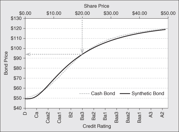
Exhibit 9.4 Synthetic versus Cash Bond

At this stage you are probably wondering how we determine the pricing relationship between a company's debt and its equity. We think about this relationship in the following way. The market value of a company's stock and bonds reflects the market value of a company's assets. When the price of the company's stock falls, the equity markets are signaling that the value of the company assets have fallen. Since the face value of debt remains unchanged, the firm becomes more levered on a market value weighted basis. As a result, the credit risk of a bond increases, and its price and credit rating falls. Therefore, there is a direct relationship between the market price of a company's stock and the market price of its debt. (For more on the technique used to derive this relationship, see the book Quantitative Analytics in Debt Valuation and Management listed in the reference section.) The gray dashed line in Exhibit 9.4 shows how the price of the five-year, 7 percent coupon bond changes as the price of the company's stock changes. The solid black like shows the same relationship for the synthetic bond. Notice how well the value of the synthetic bond tracks the cash bond. This shows that by selecting the appropriate strike, and number of spreads, a synthetic bond can provide an excellent substitute for the real thing, when none are available in the marketplace.

If we think of equity as a call option on a company's assets with a strike price equal to the face value of debt, we can extend that analogy and posit that an asset can be valued as a zero strike call on the company's assets. The performance characteristics of an option are dependent in part by the option's strike price. As a result, the performance characteristics of the cash bond and the synthetic bond will change differently as time passes. All other things being equal, the delta of a put spread will rise over time. Since the options used to replicate the cash bond are close but not perfect surrogates, the rate of drift in the delta of the options used to create the synthetic bond might move away from the delta of the options imbedded in the cash bond. As a result, the structure must be reoptimized from time to time. At a minimum, you should do this rebalancing as each coupon payment is made. This will ensure the tracking error between the cash bond and the synthetic bond is held to a minimum. While this analysis assumed volatility surface did not change over the investment horizon, a shift in the term structure or skew might allow you to restructure the synthetic bond to improve returns as well.

In this example, we showed that we are able to create a high-yield bond synthetically by purchasing Treasury notes and selling a put spread. Prices and market factors were chosen to show that you should be indifferent from owning a cash bond or a synthetic one. Returns over time will be the same. It is important to recognize that prices in the equity and options markets do not always agree with the price of risk in the bond market. This gives rise to the potential for arbitrage opportunities. With respect to the options market, this analysis shows that if the implied volatility associated with the company's stock is 35 percent, we can recreate this corporate obligation with the same expected yield to maturity. The iVol of the associated equity is a key ingredient to the valuation of the synthetic corporate bond. If the iVol used to price options for the underlying equity were more than 35 percent, the synthetic bond would cost less relative to the cash bond. If the iVol used to price long-dated options of the underlying equity is less than 35 percent, the cash bond would cost less than the synthetic bond.

The solid black line in Exhibit 9.5 shows the sensitivity of the yield to maturity of the synthetic bond to changes in implied volatility of the underlying stock. Notice that as iVol rises, the yield to maturity for the synthetic bond rises. In this example, for an increase of one vol. click, the yield to maturity of the synthetic bond would increase by 21.5 basis points. Likewise, if iVol falls by 1 percent, the yield to maturity on the synthetic bond falls by 21.5 basis points. This change in yield to maturity is equivalent to a $0.83 change in price.

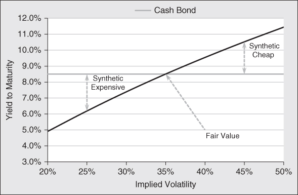
Exhibit 9.5 Valuation Comparison

This is the setup for arbitrage opportunities between these two distinct markets. We can look at bond prices to determine how the fixed-income portfolio managers and traders are pricing volatility relative to those priced by the equity options markets. This is very important for hedge funds that invest across asset classes and a company's capital structure. Since most market participants focus on just one asset class, there are times when there is a divergence of opinions between these two markets. When the bond market is discounting a lower volatility than the options markets, cash bonds will be more expensive than synthetic bonds. Under these conditions, we should sell cash bonds and buy synthetic bonds. When corporate bond investors are more fearful than the equity and option investors, they will incorporate higher volatility into their securities valuation by demanding higher yields. Under these circumstances, we should sell their synthetic bonds and buy traditional cash bonds. This is a distinct method for long-only investors to add alpha to their portfolio returns and outperform their index benchmarks. Hedge funds that seek to eliminate market risk can buy cash bonds when these markets reflect higher risk than the options market, and hedge them by buying put spreads, leaving nothing but interest rate risk. To eliminate that risk, they could sell T-note futures. This will result in a pure alpha-generating strategy, as returns will be independent of general market action. Shorting cash bonds is a bit more problematic as they tend to be harder to borrow. However, you might look to single-name CDS (credit default swaps) and buy put spreads if credit is pricing in a lower volatility than the options market.

There are some pragmatic issues that need further discussion. The typical option series for single names have an expiration cycle of 3, 6, 9, and 12 months. Corporate debt obligations typically extend for years. Industrial and financial companies often issue debt securities with 5- to 10-year maturities. It is not uncommon for telecom and utility companies to issue debt with tenors as long as 30 years. This makes using listed options somewhat problematic when creating debt securities synthetically. LEAPS (Long-Term Equity AnticiPation Securities) are a type of listed option with expirations that extends for up to three years. These options provide a viable alternative for synthetically creating short-term debt. Institutional investors who want to create debt synthetically with maturities longer than two or three years have to look to the over-the-counter market for these financial products. Since these markets are less liquid and fungible, we should expect to pay higher transaction costs to both initiate and close positions. This makes short-term arbitrage trades more difficult. These markets would be more useful for those who want to initiate positions with a longer-term time horizon.

As a final thought, you might want to use synthetic bonds for pricing bonds that trade very infrequently. Since you are simply pricing bonds and not trading synthetic bonds, one can model options with expiration dates that more closely align with the maturity of the bond. You can do this by extending the volatility surface based on what is priced in the marketplace. This way, you are matching long-term volatility expressed by the options market with that of the corporate bond in question. The term structure of volatility is generally upward sloping. It is the long-term volatility in equity prices that is priced into long-term bonds.

Final Thought

Creating hedges and synthetic securities are some of the powerful features of derivatives products in general and options in particular. In this chapter, we wanted to introduce you to the concept of synthetics which most individual investors typically do not think about in their investment activities. With the basics of synthetics under your belt, you can use your imagination to tackle investment and hedging challenges that usually go unsolved.