Chapter 10
Home Runs

The preceding chapters discussed theory, application, and strategy concerning methods to improve returns and manage risk with options. While theory is great, we need to see how some of these strategies are applied and work in the real world of investing. In this chapter, we will provide a number of real life examples of investments that are either directly expressed with options or contain imbedded options that drive the risk/return equation. Since options are leveraged investment vehicles, assets with option characteristics have the potential to generate outsized gains. Furthermore, listed and OTC options enable investors to structure investments to limit risk and create the potential for very high returns. As a good way to show the potential offered by the listed option market, we will discuss a specific example of how skilled investors structured a multileg option trade in the oil markets to make huge gains without taking much, if any, risk.

The Oil Trade

In the years after the dotcom crash and 9/11, the federal government increased spending in an attempt to increase the rate of economic activity in the United States. At the same time, the Federal Reserve eased monetary policy by significantly lowering short-term interest rates by increasing their purchases of U.S. Treasury securities for the same reason. From 2002 to 2008 the Western economies recovered modestly, while the big winners were the BRIC (Brazil, Russia, India, China) countries. Up to this point, these countries were modest consumers of oil as compared to the United States and Western Europe. With trade barriers falling, these and other emerging markets increased their manufacturing output and domestic consumption. These products were sold into the international markets and these BRIC countries grew their GDP at very high rates, some in the range of 7 to 10 percent. With manufacturing growing and international trade increasing, transportation of goods (shipping, rail, and trucking) also became a big area of growth. To transport the goods produced in Asia to buyers in the Western economies, the global fleet of container ships, oil tankers and dry bulker carriers exhibited spectacular growth. Manufacturing and transportation of raw material and manufactured goods, of course, are very energy-intensive business activities.

Twenty years ago, only a small portion of the population in developing countries owned their own cars. As local development and international trade brought fast growth in wealth in these countries, many people bought cars. The explosion in automobiles for personal transportation was particularly acute in China, for example. It was not long before traffic jams in the major cities of developing countries became legendary. At the end of the day, with an increase in manufacturing and international trade, compounded with staggering growth in local transportation, the demand for energy, particularly liquid energy, went to record levels. This brought on a boom in oil prices (see Exhibits 10.1 and 10.2).

Exhibit 10.1 Historical Price of Crude Oil

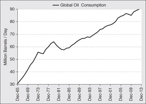
Exhibit 10.2 Historical Crude Oil Consumption

The demand for oil has grown steadily since its discovery. Exhibit 10.2 shows how global consumption of oil grew steadily since 1965. The recession of the late 1970s caused by a spike in interest rates in response to high inflation rates resulted in a reduction in economic activity and demand for energy. But once the global economy started to grow in the early 1980s, the global demand for oil has grown steadily and has not looked back. With demand for energy growing by leaps and bounds, many analysts and investors believed that investments in oil and gas would be the way to riches. For a time, this was indeed the case. Exhibit 10.1 shows the price of oil going back to 1999. Notice that the price of oil might fluctuate significantly more than consumption, but at the end of the day, they both follow a rising trend.

With demand growing rapidly along with a dearth in significant discoveries of new sources of oil, many believed that an oil shortage was just around the corner. Rising prices seemed to support that proposition. This gave rise to what became a widely followed investment theme known as peak oil. Peak oil is a concept introduced by M. King Hubbard in 1956. This theory states that every oil field goes through a life cycle. It starts with exploration, which leads to discovery. Once a field is discovered, huge investments are made to develop the production infrastructure to develop the resource. This entails drilling production wells and building a pipeline infrastructure to take oil from the fields to the refineries. As more wells are drilled on an existing field, oil production increases. It is important to remember however, that pockets of oil, while sometimes very large, ranging in the billions of barrels, are limited in size. At some point, additional wells will not increase production. As production takes oil out of the ground, pressure that once pushed oil out of the ground falls. At some point natural pressure falls away, the oil must be pulled out of the ground. From that point forward, production declines until the resource is depleted and the field produces no more oil. In short, oil production starts at zero and rises until it hits a peak, then falls back to zero. Since all fields go through this process, it is logical to conclude that the sum of all oil fields around the globe will follow the same path (see Exhibit 10.3).

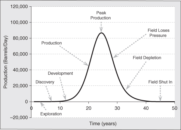
Exhibit 10.3 Oil-Field Production Cycle

Peak oil became a particular concern as oil production was far outdistancing new discoveries. If new discoveries were not going to keep up with production, it is logical to conclude that supplies would run out someday. To add weight to this theory, investors had seen peak oil theory play out first hand in the United States. There was a time when the United States was the largest oil producer in the world. Massive discoveries in the Middle East quickly moved North America into second place. By the mid-1970s, production in the United States reached a peak of almost 10 million barrels a day. From that point to the late 2000s, oil production fell by half, hitting just 5 million barrels a day by 2008.

This was not just a problem for production in the United States. In 1976, a fisherman by the name of Rudesindo Cantarell discovered a super-giant oil field off the southeast coast of Mexico. Experts estimated the field held 35 billion barrels of oil and held the expectation that about half of it was recoverable. Its development grew rapidly after discovery. By 1981, 40 wells were producing 1.1 million barrels a day. Well pressure fell rapidly and by 1994, production was down to 0.9 million barrels a day. To extract the remaining oil, 26 offshore platforms were put to work drilling nitrogen-injection wells to increase the pressure in the field. With additional production wells, PEMEX, the Mexican oil company, brought the field to peak production of 2.2 million barrels a day in 2004. While secondary recovery techniques can maintain or even increase production in the short run, doing so is the equivalent of putting the oil field on life support. It is just a matter of time before the last bit of oil is squeezed out of the field and production runs out. With the fields approaching depletion, production from this field has now fallen to less than 0.4 million barrels a day. Optimists looked to the Middle East for additional production, and they were able to do so at the margin. It takes many years of lead time and a significant investment of capital to increase the production of any field. In addition, increase Middle East production for local consumption. Since the Middle Eastern economies were growing rapidly, energy consumption in these countries was growing just as fast, if not faster, than the world as a whole. In the end, oil supplies appeared to become tighter. With this backdrop, the psychology was in place for the price of oil to move sharply higher, and it did.

Purchasing stock in exploration and production companies handsomely rewarded many investors. Oil service firms that helped develop the existing inventory of oil fields earned healthy profits as well. Since exploration and production companies own oil in the ground, buying stock in these companies is like buying a call option on the price of oil. The strike price of that option is the cost of extracting that oil and sending it to market. The cost of producing oil varies from field to field driven by unique geological and infrastructure challenges and regulatory hurdles as well. Furthermore, there are different grades of oil that affect the cost of production and refining, and the different modes of transportation have their own cost structures. So every field has a different strike price. What makes it different from a traditional option is that the time to expiration is undefined. Oil in the ground does not go away, of course. The oil company has the option to exercise it and develop an oil field whenever it thinks it can sell its oil at a price higher than the production costs. This is the point where the option goes in the money.

Assume for a moment that a company owns 1 billion barrels of recoverable oil in the ground and the estimated cost to extract and deliver that oil to market reflects the costs indicated in Exhibit 10.4.

	Reserve (millions of BBLs)	Production Cost/BBL
Low Cost	500	$30
High Cost	500	$50
Total	1,000

Exhibit 10.4 Reserves & Estimated Cost of Production

Further assume this company has no debt and there are 1 million shares outstanding. In January 2005, the market price of Brent North Sea oil, which is a global benchmark for the price of high-quality oil, was $43 a barrel. At this price, the low-cost reserves are an in-the-money option. The E&P firm can produce the oil at $30/BBL and sell it for the going rate of $43/BBL. The difference of $13/BBL goes to the company's bottom line. Given this operating leverage, the E&P firm will earn higher profits on a greater than one-for-one basis when the market price of oil rises. If for some reason the market price falls below the cost of production, the E&P firm will lose money on every barrel of oil produced. Instead of suffering this loss, the E&P firm can stop or reduce production and wait for higher prices. (One should be aware of the limits of halting production. Halting production can change the geology of an oil field, reducing its ability to produce at the same rate once the field is put back into production. For the sake of this analysis, we will ignore this complexity.) The high cost of oil represents an out-of-the-money option on oil prices. At current prices, it is not economical to bring these fields into production. Being an out-of-the-money option, once the price of oil rises sufficiently, the value of the option rises rapidly and the firm can produce very levered returns by bringing the field into production. Exhibit 10.5 is a chart of the payoff pattern of these options (gray lines) without time value. Combining these options and incorporating time value (black line) results in an estimate of total enterprise value.

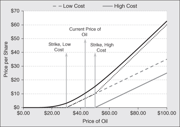
Exhibit 10.5 Equity Value Based on Imbedded Option

Since these oil fields represent options on the price of oil, we can use option-pricing theory to value the company. All we need to do is input the appropriate variables into an option-pricing formula as they relate to the oil fields and oil price behavior. To do this we apply the historical volatility of returns on oil prices of 16 percent. The next important variable is time. Engineering reports might tell us that it will take five years to produce all the oil from these fields once they are put into production, and that a field awaiting production is expected give up its reserves sometime over the next 10 years.

If oil is at $43/BBL, as it was in January 2005, the value of this company is about $10.31 a share. Options always have value. If the price of oil falls $13.00/BBL to $30, the cost of production would equal revenues. A cash-flow analysis would show that the company would not make any money by producing oil. It suggests this company does not have any value. But the option to produce has value. If we value the company as an option on oil prices, we find the value of this company falls by $7.16/share to $3.15. While the company does not make money at this price, a rational buyer would pay $3.15 for the option to produce oil. The option becomes apparent when we examine the skewness of returns. If the price of oil increases by $13/BBL to $56, the value of the firm increases by $10.03/share to $20.34. The investors make more on the way up than they lose on the way down.

This analysis uncovers a viable investment strategy. If one is bullish on the price of oil, one could buy cheap call options on oil with undefined expirations by investing in exploration and production companies that have reserves that can be brought into production relatively quickly when prices rise. Since these reserves do not produce free cash flow at current prices, they only have time value. Since they have essentially an infinite time to expiration, they will be cheaper and more flexible options than call options on oil itself. This is not just a theoretical exercise. Exhibit 10.6 is a list showing the returns on a smattering of E&P stocks, all of which showed incredible performance.

Company	Initial Price	Ending Price	Return w/Dividends Reinvested
Cabot Oil & Gas	3.58	16.93	385%
Range Resources	12.73	65.54	433
Comstock Resources	20.77	84.43	310%
Chesapeake Energy	15.47	67.36	346
Southwestern Energy	5.59	48.53	724%
Quicksilver Resources	11.71	39.2	235%
Ultra Petroleum	23.08	98.59	327%
Noble	14.56	51.40	260%
Contango Oil & Gas	6.92	92.05	1230%
Suncor	16.94	57.22	242%
Crescent Point Energy	16.85	40.38	283%
Average			434%
Oil	43.00	131.00	205%
Natural Gas	6.16	13.51	119%
Average			162%

Exhibit 10.6 Returns on E&P Companies from January 3, 2005, to July 1, 2008

At the close of trading on January 3, 2005, the price of oil was $43.00/BBL. By the end of trading on July 1, 2008, it rose to $131.00/BBL, for a gain of 205 percent. At the same time, the price of natural gas, which is a substitute for crude in some uses, rose 119 percent. Exhibit 10.6 shows us that the typical exploration and production company rose by over 400 percent. Natural gas is a byproduct of oil production. As a result, most oil producers also produce natural gas, so one should compare the performance of E&P companies with the price of hydrocarbon energy. On this basis, equities outperformed the commodity by a factor of 2.6:1. These equities did indeed behave like options on the price of oil. Contango Oil & Gas, the best-performing equity, represented an out-of-the-money option, as the company was not producing at all in 2005. By 2008, it had put a field into production and had a revenue run rate of $117 million a year. Bear in mind these companies have compound option features that go beyond the option to produce oil. Many of these companies employ financial leverage by issuing debt. In the discussion on synthetics in Chapter 9, we explained that when a company issues debt, equity becomes an option on company assets. In some sense, the equity of an exploration and production company is an option on a portfolio of oil call options. This expresses itself in the highly levered returns displayed above. When investing in E&P companies, one must be very careful to understand both the cost of producing reserves and the company's capital structure. When the price of oil falls, the price of E&P stocks will fall just as fast as they rise.

Although this is an excellent example of how equity in an E&P stock is like a call option on the price of oil, an example of equal interest centers on the action of oil options before and during the oil price crash that occurred in the six months after its peak. In 2008, the term structure of volatility was inverted. This is a natural occurrence after a very volatile movement in the price of an asset. Investors expect volatility to continue in the near term, but at the same time expect volatility to revert to the long-term mean over time. One of the interesting aspects of all commodities is that the inflation-adjusted price reverts to the long-term average over time as well. Historical experience tells us that volatility on all asset classes exhibits a mean reverting property. The only question is how long it will take for the mean reversion to take place. Exhibit 10.7 is a chart of the term structure of implied volatility on oil options in the months before the price of oil peaked.

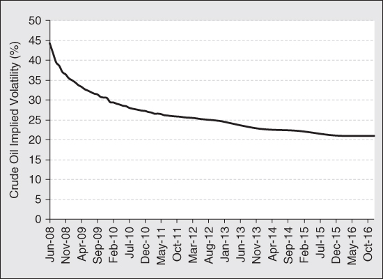
Exhibit 10.7 Crude Oil Volatility Term Structure, May 2008

The typical term structure of volatility is upward sloping. Investors tend to have a better understanding of risk in the short term relative to the long term. When the term structure inverts, the market provides an opportunity for those who want to carry a volatility arbitrage trade through a calendar spread. In this trade, the investor sells short-dated volatility high and buys long-dated volatility more cheaply. When the trade is weighted on a delta-neutral basis, the investor earns a profit if short-dated iVol falls relative to long-dated iVol. How this occurs is important, however. We showed in Chapter 4 that this structure is long vega. As a result, the investor will gain if the volatility curve flattens with an upward shift in volatility across all expirations. The investor will also enjoy a profit if short-dated volatility falls while long-dated volatility holds steady. Losses will be suffered if volatility falls across all expirations or the curve inverts further. The structure is also short gamma. As a result, if the price of the underlying trends in one direction or another, the investors will suffer a loss. Since the structure is short gamma, it will be long theta. Therefore, the structure will increase in value as time passes, should the price of the underlying security and implied volatility stagnate.

With so much uncertainty about the future price of oil, the skew chart of oil took the shape of a “smile.” Options that are out of the money are priced at a higher iVol than those close to or at the money. The smile shape in the skew chart generally occurs when speculators and option writers expect big price movements, but are uncertain about which way that price jump will go.

Exhibit 10.8 shows the skew chart for 3-month and 24-month options on crude oil. When presented with a volatility smile, one can sell iVol expensively by selling out-of-the-money options while buying at-the-money options on a delta-neutral basis. One way to do this is to sell out-of-the-money put and call spreads. If skew flattens, this strategy will be profitable. This strategy carries positive theta so time is our friend in this strategy. To offset theta, the trade is short gamma, so the trade will show a loss if the price of the underlying trends in one direction or the other.

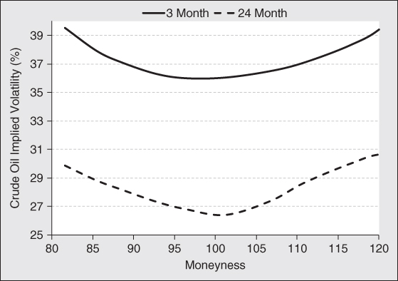
Exhibit 10.8 Crude Oil Volatility Skew, May 2008

The combination of an inverted term structure along with a volatility smile presents an opportunity to create a very cheap and even free straddle. The options on crude oil provided such an opportunity in the months before the oil price peak and eventual crash. The clues to create a free straddle in May of 2008 were revealed above. To buy volatility cheap, buy long-dated at-the-money puts and calls on a delta neutral basis. This is the lowest point on the volatility surface. At the same time, sell short-dated out-of-the-money put and call spreads. These are the highest points on the volatility surface. These out-of-the-money spreads offset the time decay one suffers on the long-dated options. Exhibit 10.9 shows the structure of this multileg trade.

Type	Put	Put	Put	Call	Call	Call	Combo
# Buy or Sell	1	−1	1	0.57	−1	1
Strike Price	95	102	110	119	134	145
Risk-free Rate	1.80%	1.80%	2.50%	2.50%	1.80%	1.80%
Dividend	0%	0%	0%	0%	0%	0%
Time to Exp. (Mth)	3	3	24	24	3	3
Volatility	37.10%	36.30%	26.65%	26.75%	37.10%	39.00%
Price	$1.50	$2.96	$11.88	$17.77	$2.65	$1.45	$19.33
Delta	(0.13)	(0.23)	(0.33)	0.59	0.23	0.14	0.00
Gamma	0.010	0.014	0.008	0.009	0.014	0.010	0.00
Vega	12.1	17.2	59.0	63.1	17.5	12.6	84.9
Theta	(8.70)	(11.96)	(2.67)	(5.46)	(13.44)	(10.12)	0.80

Exhibit 10.9 Crude Oil Trade Structure, May 2008, Crude at $114.56

At first blush, one might say this is not a free straddle. After all, one has to pay $19.33 up front. But remember, the cost of an option is not necessarily the amount of money you pay up front. The cost of an option is the value it loses as it ages. There is an interesting aspect to this structure. It starts out gamma neutral and nearly theta neutral, so one should not expect the structure to lose value over a short investment horizon. Furthermore, one is able to take advantage of rolling up the inverted term structure as time passes. The vega of the long-dated options is far higher than the short out-of-the-money put and call spreads. Consequently, the value of the spread will rise as it moves toward the forward volatility surface.

Exhibit 10.10 shows a total return analysis of this multileg trade. The solid black line shows the return profile for an instantaneous change in the price of crude oil. Since the structure is initially delta and gamma neutral, the return profile is flat for a moderate change in the price. As it drifts further away, gamma becomes positive, creating the return characteristic of a straddle. The gray dotted line shows the expected return for the structure, assuming volatility moves toward the implied forward volatility surface. Since the structure is vega positive and iVol is expected to rise due to the inverted term structure, this multileg trade is expected to increase in value by $0.26 at a minimum. After transaction costs, this is a free straddle.

Exhibit 10.10 Total Return Analysis

The black dot on the chart above shows the actual profit one would have earned by holding this trade for a one-month time horizon. It performed even better than expected as the iVol for long-dated at-the-money options actually increased by two vol. clicks. Remember, a free straddle does not mean a riskless straddle. Once delta was hedged out, this became a volatility trade. It would perform best if either iVol increased or the price of crude oil trended in one direction or another.

This is not just a theoretical trade discovered after the fact. In our market-making activities, we witnessed a large hedge fund put this trade in the second quarter of 2008. The fund making this trade was a bit early, and they had to roll the position for a few months. But rolling up the volatility term structure meant they were being paid to wait for a bearish resolution to the oil price spike. When investors recognized that peak oil was not at hand, the price of crude oil finally cracked. The gains captured by this trade were ultimately enormous. This is a terrific example of the power of a free option. Since one does not have to suffer time decay, sophisticated professional investors can place a trade “in size,” without the risk of significant loss if they have to wait for the market to move in their direction. The moral of this story submits that if you can find a free option or straddle, take it.

Warren Buffett and Berkshire Hathaway—Selling Puts and Buying Calls

Many think of Berkshire Hathaway as a holding company that possesses a number of wholly owned subsidiaries that engage in a wide variety of business activities. From the standpoint of organizational structure, this is indeed the case. At its core, Berkshire is a property and casualty insurance company. In its primary insurance activities, it assumes the risk of loss for people and organizations that are directly subject to certain risks. P&C insurance protects businesses and people against losses to their business, home, car, or other assets and personal heath as well. It also covers these entities against legal liabilities that might result from personal injury to people or to the property of other individuals. In its secondary insurance business, it provides reinsurance. A reinsurance contract is another form of risk transfer. Reinsurance is simply a contract where one insurance company, the direct insurance provider, offloads some or all of the risk of an insurance contract to another insurance company. In addition, Berkshire provides financial protection through life insurance and financial guarantees. Insurance companies protect themselves through diversification. They write insurance contracts against a wide variety of risks to a large number of customers who are spread out by both geography and industry. By diversifying across type of risk, customer, geography, industries, and so on, losses within any given time period are predictable and do not put the enterprise at risk of excessively large losses or insolvency.

The beauty of P&C insurance is that the customer pays a premium up front for protection against a future event. While this creates a liability for Berkshire, it also provides cash that it can invest to produce additional revenue. Warren Buffett has proven himself to be one of the best investors of all time, and this has been a key to the success of Berkshire. Mr. Buffett likes stocks for the long term, so much so that he typically buys companies outright. These investments become permanent subsidiaries of the enterprise. We are not aware of any company that Berkshire has purchased outright that was later sold.

If we look at Berkshire from the perspective of options theory, we see that Berkshire is in the business of both selling and buying options, and collecting and paying premium. At its core, insurance is a put option. This put option, however, is one unlike the typical option discussed in this book that pays if the price of an asset falls. The put option sold by a P&C insurance company pays if something breaks. By writing insurance, Berkshire collects premiums to cover the costs of catastrophic events that might occur in the future. Think of homeowner's insurance as a put option on the risk that the house is burned down or a tree falls through the roof. With that premium collected by selling insurance, Berkshire buys call options in the form of common stock. As discussed in Chapter 9, common stock is a call option on the assets of a corporation. If the value of the assets rises, the value of the stock rises. If, on the other hand, the value of the company's assets falls below the face value of the company's debt, the company goes bankrupt. The owners of common stock lose everything. This is another way of saying that the option expires worthless. This has happened at Berkshire. When Mr. Buffett purchased Berkshire Hathaway, it was a textile company. As time passed, it became clear that it was a dying business so Mr. Buffett wound down that enterprise and eventually closed it as he repositioned the enterprise into what eventually became a holding company.

At the end of the day, Berkshire Hathaway is an enterprise that sells puts and buys calls as its core, fundamental business strategy. Berkshire has been successful in this endeavor and provided shareholders with outsized returns by purchasing underpriced call options and selling overpriced put options. From this perspective, the secret of Mr. Buffett's success is that he only sells puts when he believes they are expensive and buys calls when he believes they are cheap. In the reinsurance business, for example, there is a clear premium cycle. If there are no hurricanes in Florida or no earthquakes in California, competitors in the P&C space become complacent and succumb to the pressure of growing earnings in the short term. As a result, reinsurance premiums fall. At this point in the pricing cycle, Berkshire does not write reinsurance. Mr. Buffett goes so far as to continue to pay the reinsurance staff well during these periods to remove the incentive to do business for business sake. Nature does what it will and hurricanes strike and earthquakes hit. Those companies that sold insurance too cheaply suffer outsized losses relative to the premium collected when those events occur. With a drop in their capital base, they lose the ability to write new insurance policies and become insignificant competitors in the marketplace. Furthermore, companies who maintain a strong capital base become more fearful of natural events and cut back on writing new insurance policies. This is the point where Berkshire becomes an aggressive seller of reinsurance policies. Other companies run swiftly to remove risk from their books and are willing to pay a high price to do so. In the world of options, this is the same as selling puts when implied volatility is high. At the end of the day, Berkshire only sells puts when iVol is high and does not participate when iVol is low.

Berkshire follows the same philosophy with regard to its investments. Stock prices rise and fall with the economy and investor sentiment. When investors are feeling good, they push stock prices up to extremes to the point of overvaluation. At this point in the cycle, Mr. Buffett will reduce his holdings of common stocks and let cash build up on the balance sheet, keeping it available for the day when prices are more reasonable. Since stock is an option on company assets, and the value of that option is dependent on iVol, high share prices imply high risk. On the flip side, when share prices are depressed, the iVol implied by a company's equity is low. This is the point where Berkshire buys options on company assets (i.e., equities).

At the end of the day, Berkshire sells insurance (i.e., puts on catastrophe) when iVol is high and shows the discipline to stand aside when iVol is low. Likewise, Berkshire buys equities (i.e., call options) when iVol is low. In this way, Mr. Buffett systematically sells volatility high and buys it low. The importance of this strategy goes further and speaks to diversification. There is no statistical relationship between the cost of insurance and the value of financial assets. As a result, there is no connection between when insurance benefits will have to be paid and the performance of equities. Since there is no correlation between the financial performance of the puts written and the call purchased, risk is reduced.

There is another way Berkshire buys calls on company assets. It sells naked puts outright. Between the years 2004 and 2008, Berkshire sold out-of-the-money put options on the S&P 500, FTSE 100, Euro Stoxx 50, and the Nikkei 225. According to the 2012 10-K, the notional value of those options is close to $34 billion. It is difficult to tell what iVol was used to price the individual contracts or times to expiration when selling these puts, but we estimate Berkshire took in approximately $7.25 billion in premium (give or take a billion) when they originally made the sale. It is our understanding that Berkshire sold out-of-the-money puts. If they took advantage of skew, which we are sure they did, they would have sold those options with an iVol in the low 20s. Since realized volatility on large-cap stocks in developed countries runs in the mid-teens, it looks like Berkshire was able to sell expensive puts, which expire between 2018 and 2026. Bear in mind that Berkshire is selling puts on a buy-and-hold basis. The regulatory filings stated that Berkshire expects these index puts to decay in value over time and potentially expire worthless. In short, they are selling price insurance with the hope and expectation that a claim will never be filed against the insurance contracts.

Put–call parity tells us that selling cash covered puts is like buying a covered call. We see this by rearranging the equation presented in Chapter 9.

If, for some reason, markets fall dramatically, Berkshire has the financial resources and liquidity to take ownership of the underlying stocks that populate the indexes, so it is reasonable to assume the puts are covered with cash or equivalents. Since this is equivalent to a covered call strategy, Berkshire is selling covered calls to produce income. Since it looks like they were able to do so with an iVol higher than historical rVol, the strategy should produce excess returns. This is precisely what Berkshire has done as it sells put options. Remember that Berkshire is selling puts on a sell and hold basis. As a result, one should expect this trade to produce positive alpha as the analysis in Chapter 4 suggests.

The moral of the story is this: We can describe Berkshire Hathaway as a portfolio of options. The company systematically sells expensive options and buys cheap ones. Over time, this is a winning strategy.

The Louisiana Purchase—The Greatest LBO of All Time

We know from corporate finance theory that equity is akin to owning a call option on the underlying asset. If there is no debt associated with an asset, the option is deep in the money and one can value that asset as a zero strike call. If there is debt associated with the asset, the strike price of the call is equal to the value of the debt used to finance the purchase of the asset. Most companies have debt levels that are a fraction of the value of the asset. Equity in these firms is simply a deep in-the-money call. If the value of debt is equal to the value of the asset, the equity represents an at-the-money call on those assets. There are times where the face value of debt is greater than the market value of the asset. Prior to the financial crisis in 2008, there were many lenders who would provide mortgages on houses that exceeded the value of the property by as much as 20 percent. In this case, the homeowner held an out-of-the-money call option on the property they lived in. Other times, a business will languish and the value of the company's assets will fall below the face value of the company's debt. The company will be able to remain in business and continue operations so long as they can make their debt payments. In these circumstances, equity in the real estate or business described earlier represents an out-of-the-money option on the value of the asset with an undefined expiration date. To keep that option alive, the owner of equity must continue to service the debt. One can think of this debt service payment as option premium. Thought of in this manner, the Louisiana Purchase was the greatest LBO and cheapest option purchased of all time. The story of this transaction is quite interesting and investors should keep it in the back of their minds when allocating capital.

The land covered by the Louisiana Purchase encompasses an enormous parcel of land that represent what are now 15 states in the United States. Specifically, the Territory of Louisiana covered all of present-day Arkansas, Missouri, Iowa, Oklahoma, Kansas, and Nebraska. The territory also covered parts of what are now Minnesota, North Dakota, South Dakota, New Mexico, Texas, Montana, Wyoming, Colorado and Louisiana. A small portion of the land extended into what are now the Canadian provinces of Alberta and Saskatchewan. This territory covered a grand total of 828,000 square miles, a very serious piece of property in deed.

Exhibit 10.11 The Louisiana Purchase

Source: The History of American Business, historybusiness.org

From 1699 to 1762, the government of France owned a vast area of land that was then called the Territory of Louisiana. At the end of the Seven Years' War, France gave the territory to Spain, a key ally of the state. The city of New Orleans is located at the mouth of the Mississippi River, making it a key shipping port for agricultural products that were transported to other parts of the United States. In 1795, Spain and the United States signed the Pinckney's Treaty, which gave U.S. merchants the “right of deposit.” The right of deposit gave U.S. merchants the right to freely navigate the Mississippi River and store goods, such as flour, tobacco, pork, feather, cider, butter, cheese, and so on for export. This treaty was short lived and Spain revoked it in 1798, greatly upsetting relations between the two countries. In 1801, the right of deposit was restored.

But in 1800, Napoleon Bonaparte signed the Treaty of San Ildefonso with Spain to take back the territory as he set his sights on building an empire in North America. This treaty was kept secret until November 3, 1803, which was just three weeks before France and the United States ultimately cut a deal to transfer ownership.

Getting a deal done was anything but certain. Thomas Jefferson, who was president at the time, recognized the geographic significance of New Orleans, and in 1801 he sent representatives to Paris to make an offer to buy the city and port of New Orleans from the French government. Given Napoleon's ambitions, it was no surprise that he rejected the idea. In 1803, negotiations began anew. Pierre Samuel du Pont de Nemours, a French nobleman, facilitated negotiations with France at Jefferson's request. It was at this time that the idea of a larger Louisiana Purchase was put forth. At the same time, France was under financial pressure as Napoleon began preparations to invade Britain in 1803. Furthermore, there was a slave revolution going on in Saint-Domingue (modern-day Haiti). Napoleon had sent more than 20,000 troops to reconquer the territory and reestablish slavery. But yellow fever and the revolutionaries destroyed the French army, in what became the only successful slave revolt in the Americas. Without the revenues from the sugar trade, Louisiana was not so attractive to the French empire. Even though Spain had not completed the transfer of Louisiana to France, Napoleon decided to sell the entire territory to the United States. Napoleon liked the idea of selling something that was not his yet, and the sale would also serve to raise cash to fight the imminent war against Britain. The Americans were prepared to pay $10 million for New Orleans and the surrounding area, but were pleasantly surprised when France offered the entire territory for $15 million.

Complicating the deal still further, many in the United States, led by House Majority Leader John Randolph, as well as some historians, believed that this purchase was either unconstitutional or simply unjust. Jefferson's political adversaries made hay of the fact that a strict constructionist would appear to play fast and loose with the constitution. James Madison, one of the authors of the U.S. Constitution was thrown into the same camp. The House even went so far as to hold a vote to deny the purchase, but it failed by two votes, 59–57. The Federalists feared that the Louisiana Purchase would alter the balance of power. They felt the purchase was a potential threat to Atlantic seaboard states, merchants, and bankers, shifting power and influence to the Western merchants and farmers. Furthermore, an expansion of the number of slave-holding states would inflame already existing divisions between the northern and southern states. Jefferson argued that such a purchase was constitutional under the power granted to the president to negotiate treaties. Finally the question of citizenship was an issue. The treaty between France and the United States granted citizenship to the French, Spanish, and free black people living in New Orleans. Critics of the deal felt that foreigners, who were unacquainted with the U.S. style of democracy posed a risk to the political system. In the midst of all this, the government of Spain argued that Napoleon did not have the legal authority to sell the territory. They argued the Third Treaty of San Ildefonso forbade it and that France promised Spain it would never sell or alienate Louisiana to a third party. Furthermore, Spain argued that if the property were to be transferred, it must be transferred to them. But in the end, the Spanish prime minister had authorized the United States to negotiate with the French government for the acquisition of territories, which suit U.S. interests. But in the end, the path was cleared for the federal government of the United States to purchase the territory, the Senate ratified the treaty and the two houses of Congress authorized the funds needed to close the deal.

Not surprisingly, the federal government did not have cash on had to close the deal. As a result, the Louisiana Purchase was a highly leveraged deal. The federal government allocated $3 million of gold to the transaction and borrowed $12 million by issuing bonds underwritten by Francis Baring and Company and Hope and Company of Amsterdam. Recall that equity is an option on the underlying asset. By issuing a high degree of debt, Jefferson created an option that was slightly in the money with an indeterminate time to expiration. The U.S. government could keep this option alive by simply making its debt service payments as contracted. When the debt came due, they could simply roll over the loan and keep its option alive. Should for some reason, the government decide the territory was of little value, they could default on the loan and transfer the property to the lenders. This is akin to letting the option expire.

The moral of this story is quite simple, but one that is often forgotten. Napoleon's warmongering put him in a financial bind. In some sense he was facing the mother of all margin calls. To meet this margin call, he had to sell assets. Jefferson recognized a distressed seller of an asset that would be of tremendous value to the United States for both economic and national security reasons. Since he did not have enough money to purchase the property outright, he purchased an real option with an infinite life on the asset. It turns out the $3 million option turned into an asset worth trillions. Move over Warren Buffett, Benjamin Graham, and George Soros. It looks like Thomas Jefferson was the greatest investor of all time.

Bitcoin

Bitcoins are a new phenomenon that is just starting to get the attention of the general population. The concept of Bitcoin is quite interesting. It is a digital or virtual currency that employs peer-to-peer technology, implemented over the Internet, to facilitate instant payments. This is similar to how traditional currency works when people buy products over the Internet and pay with a debit card. To ensure transactions take place in a safe and secure manner, the sender encrypts the payment messages, which are then decrypted by the receiving entity. Anyone who intercepts the message will be unable to decipher its contents. What makes a Bitcoin transaction unique is that the workings of the system are decentralized. Traditional financial institutions do not facilitate the transaction in any way. Since a third party cannot monitor transactions, these digital transactions are anonymous, much like a traditional cash transaction with paper currency.

Bitcoins are held in a program/file that resides on one's computer. The owner of this program makes payments by sending the digital currency to the payee. Processing a Bitcoin transaction takes place on secured servers called Bitcoin miners. These servers confirm transactions by adding them to an encrypted global ledger. The payee receives his Bitcoins when his electronic wallet accesses the Bitcoin peer-to-peer network and synchronizes with the ledger. Once the Bitcoins are stored in one's wallet, they are immediately ready for use.

Bitcoin miners are paid a fee for participating in this process. In theory, anyone with the proper software can act as a Bitcoin miner and facilitate a transaction. To earn the right to process a transaction, the Bitcoin miner must perform a very difficult mathematical task. The miner who completes this task first generates a sequence of numbers that provides proof the miner solved the mathematical task. This sequence of numbers is known as “proof of work” and is attached to the transaction message. In this process, some Bitcoins, or fractions thereof, are created and deposited into the wallet of the Bitcoin miner. This is how Bitcoins are created. One does not necessarily have to perform work or sell a product to obtain Bitcoins. Like any currency, one can buy Bitcoins by exchanging their traditional currencies (U.S. dollars, euros, yen, etc.) for them. This is where a traditional financial institution comes into play. To buy Bitcoins, you need to wire money to a Bitcoin exchange. They will buy Bitcoins on your behalf at the market price and send them to your electronic wallet. If you want to sell your Bitcoins, you send them to an exchange where they are converted to traditional currency, which is wired to your traditional bank account.

To be sure, Bitcoins are a form of currency. As a result, they represent a financial asset. The value of that asset is difficult to determine, as they are not backed by anything real. Bitcoins only have value to the extent that someone will take them as payment for the delivery of a particular good or service, or to the extent someone is willing to buy them with a traditional currency. This, by the way, is true of all traditional fiat currencies. If Bitcoins are a currency, how can they have option value? To understand the option value in Bitcoins, we need to introduce the idea of a “real option.”

In this book, we discussed at length options as financial assets. There is another broad type of option known as a real option. Real options are characterized by a choice that is only available to a particular business or person in the real economy. They are not derivative instruments per say, as they represent an actual option to change course in the real world. Real options get the name “real” because they usually pertain to tangible assets (e.g., capital equipment), not financial assets.

The definition of a real option is similar to the definition of a derivative instrument. It is the right, but not the obligation to acquire the present value of a stream of cash flows by making an investment on or before the opportunity ceases to exist in an uncertain environment. This definition might be confusing. Think of it as buying an asset and deciding how best to monetize that investment sometime later. The potential for choice creates an asymmetry in potential outcomes, which creates the option's value. The following are examples of real options:

• Building a new, highly efficient manufacturing plant. When a company builds a new plant, they have the option to expand production or to close down an older and less efficient plant. By doing so, the company is well positioned to address an increase or decrease in demand, or compete more aggressively on the basis of price.
• Building a power plant that has the ability to deliver electric power to more than one electrical grid. Most power plants are connected to just one grid. They have to sell electricity at whatever the going rate is for that market. If a plant is able to locate close to a node between grids, they have the option to deliver power to the grid that pays the highest price. This choice increases the profitability of the power facility.
• A computer manufacturer designing its products to use generic off-the-shelf components enables them to have multiple suppliers of logic and memory chips, microprocessors, and other components, is a real option. It allows them to buy parts from whoever can deliver them most cheaply, at the highest quality, and in the timeliest manner.

While it may not be readily apparent, in its infancy, Bitcoins were clearly a real option in the currency space. In 2008, an unknown person by the name of Satoshi Nakamoto published a paper over the Internet describing the Bitcoin protocol. At this stage, Bitcoin was just a concept. In 2009, the concept started to take shape when a network came into existence by the release of the first Bitcoin client and the issuance of the first coins. The client was open source, which allowed anyone interested in viewing and improving the code to do so. An important feature of open-source software is that it technically does not have an owner. Anyone can work with some or all of the code to make new software. Like the original software and source code, this new and improved software is then made available to anyone for free. At the end of the day, the open-source platform allows the ecosystem of freelance developers to make and improve software for the good of the community. There are no owners, sponsors, or monopolies to extract economic rents from the universe of users.

This environment is the perfect backdrop for a real option as it is an asset with an unknown value and potential but unknown use. If someone buys a Bitcoin, she is taking advantage of an investment opportunity today in a highly uncertain environment, which may or may not have any value in the future. In 2009, Bitcoins were nothing more than an interesting theoretical currency experiment. Nobody knew what a Bitcoin was worth, if Bitcoin would become accepted as a medium of exchange in the future, or if they would represent a store of value. Since Bitcoins were in their infancy, formal exchanges did not exist where one could trade goods, services, or other traditional currencies for Bitcoins. The first transactions were negotiated in 2010 on talk forums. In these forums, those who wanted Bitcoins expressed an interest to buy them and those who had them expressed an interest in selling them. With a little give and take, they agreed on a price and an amount and transactions took place. This all took place without a controlling financial institution or controlling authority. In August 2010, a mammoth vulnerability in the protocol was identified and exploited. Over 184 Bitcoins were generated and captured by two addresses on the network. With the ability to generate (i.e., counterfeit) great numbers of Bitcoins, they would have no value. Fortunately, this flaw was identified within hours and erased from the transaction ledger. Technical changes were made to the network protocol to ensure this flaw was fixed permanently. This event added more uncertainty to the concept of a cryptocurrency. There are millions of very clever people out there who will challenge any system that attracts their attention.

The total value of an option is equal to the sum of its intrinsic value and its time value. It is fundamentally clear that if Bitcoins are vulnerable to counterfeit, then their intrinsic value is questionable. Furthermore, it was unclear if anyone in 2010 would accept them in exchange for goods and services, or for traditional currencies. It was entirely possible that Bitcoin would have nothing more than a small cult following, never making it to the mainstream. One of the first notable transactions took place when someone bought a pizza for 10,000 BTCs. Bitcoin began to gain traction in 2012 when Wikileaks began to accept Bitcoins as donations. As other organizations joined the bandwagon, the Electronic Frontier Foundation stopped accepting Bitcoins because of legal concerns. This threw additional uncertainty into the market and Bitcoin could have died then and there before it ever got off the ground. Adding additional resistance was Jim Cramer, the widely followed host of CNBC's Mad Money TV show. In an episode of The Good Wife he played himself in a courtroom scene where he stated that he did not believe that Bitcoin was a legitimate currency. With all these headwinds, it was clear that Bitcoins probably did not have any intrinsic value.

The other source of value that contributes to the price of an option is time value. While it was unclear that Bitcoin would become anything more than an interesting curiosity, there was always a chance it could become something. With time, the imperfections and resistance to a cryptocurrency might be overcome. It is time value that makes an option different from other financial assets. With respect to a financial option, one can buy an out-of-the-money option to have the right to buy or sell something for a small premium within a given period of time. With respect to a real option, one has the right to make a choice to do something sometime in the future. The significant difference between the two pertains to time to expiration. Real options do not necessarily expire. After investing in an asset with an uncertain value in an ever-changing environment, the investor retains a strategic option to change course over the life of the investment.

Take, for example, a company that buys a large piece of land and puts a small factory on that property. If demand stagnates, it has the option to do nothing. If demand increases, it has the option to expand capacity to fulfill that demand. That option will never expire so long as the company owns the land.

Back in 2008 to 2012, Bitcoins represented a deep out-of-the-money option. In the fourth quarter of 2010, you could have bought a Bitcoin for a tiny premium of about $0.08. If you held that coin, you would have had the option sell it at a later date or exchange it for a good or service if—and it was a big if—other economic actors decided to accept Bitcoins as payment. If the whole idea of Bitcoins faded away, those options would fade away, and the Bitcoin would simply become worthless. Since there was no formal exchange to trade a Bitcoin to someone else for a traditional currency, and traditional retailers did not accept Bitcoins for payment of goods and services, there was no intrinsic value to this option. But there was always the chance those mechanisms could develop in the future. If they did, you could exercise that option by trading your Bitcoins.

As it turned out, there was another option that Bitcoin proponents advertised. That was the option to hold purchasing power outside the banking system. This option does not have any value if an exchange does not develop or Bitcoins do not become a medium of exchange for goods and services. Think of this as a barrier option. Once a barrier is breached, the option can be exercised. This may not seem important, but this option became valuable at the onset of the second phase of the European banking crisis, which began in 2011. At this time, the Greek economy was falling into depression and it was becoming clear that the central Greek government was bankrupt. Greek banks were the biggest lenders to the local government, bankrupting these institutions as well. Since the Greek government could not bail out the banks, it became fundamentally clear that depositors were in trouble. This caused a run on the banks as depositors took their money out of local institutions and placed them in banks domiciled in the United Kingdom, France, and Germany. At the margin, some people took their money out of the banking system by exchanging their euros for Bitcoins. A few keen observers saw this phenomenon as well and bought Bitcoins. This caused the price of Bitcoins to rise to the $30 range by June of 2011. This was made possible because by this time, there were a number of exchanges available that would facilitate the purchase and sale of Bitcoins. Investors were putting value on the opportunity to take money out of the banking system for safekeeping as the traditional financial system was teetering on insolvency.

The established intergovernmental and monetary authorities were able to stabilize the Greek banking system and the fear of a collapse of the banking system went away. Since there was not a well-defined economic ecosystem for people to exchange their Bitcoins for goods and services, owners of Bitcoins had to sell them to buy the things they needed. As a result, the price of Bitcoins fell to just a few dollars a coin. The option to keep money out of the banking system had lost much of its luster. This did not last long.

In 2013, the banking system in Cyprus collapsed. Instead of a government sponsored bailout of banks and the banking system, the monetary regulators opted for a bail-in. This was a process in which depositors were forced to convert some portion of their deposits into the stock of worthless banks. In this process they lost money. Fearing the banking system once again, many people in Cypress tried to get their money out of local banks and, indeed, the country. Some took their money out of the banking system by purchasing gold and silver and tried to get those precious metals out of the country. Once again, there were some people who took a different approach to get money out of the banking system. They bought Bitcoins. This time, the price of Bitcoins rose to a price of $230 in April 2013. As the crisis in Cypress began to resolve itself and the need to get money out of the banking system subsided, the price of Bitcoins once again fell into the mid-$70 range. As of August 2013, Bitcoins were trading around $120.

The market price of Bitcoins is not likely to fall to the price they held in their early days because a number of issues have been resolved. Barriers have been crossed and the barrier option is now exercisable and in the money. There are now close to 40 online exchanges where people can convert traditional currency into Bitcoins. Regulators are taking a kinder eye to the currency alternative as well. Many exchanges are registering with FinCEN, the Financial Crimes Enforcement Network, which is a bureau of the U.S. Department of Treasury. This is giving regulators confidence that these important participants are taking their fiduciary responsibility seriously. In addition, more companies are beginning to accept Bitcoins as payments. As this system of cryptocurrency gains wider acceptance, it will become increasingly difficult to ban it altogether.

At the end of the day, Bitcoins turned out to be one of the great options trades in modern time. One could have bought Bitcoins in 2011 at $0.08 apiece as an option on a new currency system and shield from a shaky banking system. With perfect timing, one could have sold that option for $230 a Bitcoin. This would have provided a return of over 287,000 percent. Said another way, if you bought $100 of Bitcoins, you could have sold them for $287,500. These returns are the dream of every option traders. As of November 2015, Bitcoins change hands at about $400 a virtual coin.

Final Thought

In this chapter, we showed a few examples of how one can generate tremendous wealth by understanding the options imbedded in various securities or by simply purchasing underpriced options and selling overpriced ones. This is how many traditional businesses such as insurance companies make their money. Businesses that maximize flexibility are, in fact, buying cheap real options that enable them to change course on a dime to maximize cash flow and profits. Every once in a blue moon, a huge investment opportunity comes around that contains a very cheap option. Understanding that option is key to recognizing the opportunity. The lesson from this chapter is quite simple. Analyze businesses and individual investment opportunities as if they were options. This will reveal their true character. If there is an investment that does not have optionality imbedded in it, find a way to structure the transaction to limit downside risk while enjoying unlimited gains. Make your own option.