Confronting Inequality: How Societies Can Choose Inclusive Growth

OVERVIEW OF TECHNICAL WORK

The empirical analysis in this book is concerned with (1) the drivers of inequality, particularly economic policies; (2) efficiency/equity trade-off, which requires that we also look at drivers of growth; and (3) the links among inequality, growth, and redistribution (the difference between gross and net measures of inequality). Much of our empirical work therefore takes the form of regressions where either inequality or growth is the dependent variable and various economic policies are among the independent variables. In the case of (3), the dependent variable is growth and the main independent variables of interest are inequality and redistribution. The exact form of the regressions varies across chapters depending on the particular needs of the chapter. In this Technical Appendix, we first summarize the main empirical methods used in each chapter, and then take a detailed look at the specific regressions and results that underlie the figures in the book.

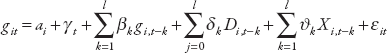
In chapter 2, we try to determine the robust drivers of inequality. The empirical framework used is the following:

where I denotes inequality over the period [t, t+5], measured by the Gini index of market (net) inequality; α_i and γ_t are country and time fixed effects, respectively; and X is a set of drivers or determinants. The equation is estimated using weighted-average least squares, which is a standard way of establishing which determinants are truly important in explaining the behavior of the dependent variable.

Chapter 3 establishes a key result of the book: inequality raises the odds that a growth spell will come to an end. A lot of the technical work in this chapter is therefore concerned with measuring growth spells by using statistical procedures to identify structural breaks in growth. The other technical exercise in this chapter is modeling how the hazard rate—the probability that a spell will end—depends on factors such as inequality. Chapter 9 uses similar methods because it too is concerned in part with determinants of the duration of growth spell, in particular whether redistribution matters. This chapter also has regressions where the dependent variable is growth (rather than the duration of growth spells) and the independent variables include inequality and measures of redistribution.

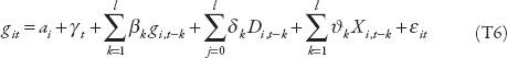
Chapter 4 studies how various structural reforms affect inequality and growth (taking into account the impact of inequality itself on growth, as established in chapter 3). To assess the direct effect of reforms and inequality on growth, we use standard dynamic (convergence) growth regressions of the form

where y_i,t is the log of per capita GDP of country i at time t,

is the average of the structural reform indicator between time t–4 and t,

is the level of inequality averaged between time t–4 and t, while

represents other controls also averaged between t–4 and t. Analogous inequality convergence regressions are run to assess reforms’ effects on inequality:

where Gini_i,t is the Gini coefficient for market inequality of country i at time t,

is the average of the structural reform indicator between time t–4 and t, while

represents other controls also averaged between t–4 and t.

Chapters 5, 6, 7 are detailed analyses of the impact of specific policies—capital account liberalization, fiscal consolidation, and monetary policies, respectively—on inequality and output. In chapter 5, the autoregressive distributed lag model is used to assess the dynamic response of inequality in the aftermath of an episode of capital account liberalization. The equation is:

where the dependent variable g_it is the annual change in the log of output (or the Gini coefficient) and D is the index of capital account liberalization. Full sets of country-fixed and time-fixed effects denoted by α_i and γ_t are included. Second, impulse-response functions are used to describe the response of output and inequality to capital account liberalization. The shape of these response functions depends on the value of the δ and β coefficients. For instance, the simultaneous response is δ₀, and the one-year-ahead cumulative response is δ₀ + (δ₁ + β₀δ₀).

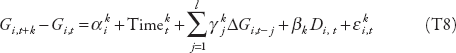
In chapters 6 and 7, a local projections method is used to assess the response of inequality and growth to episodes of fiscal consolidation. The equation is:

where the dependent variable g_it is the annual change in the log of output or the change in some measure of inequality; MP_i,t is either the fiscal consolidation episode (in chapter 6) or the exogenous monetary policy shock (in chapter 7). Full sets of country-fixed and time-fixed effects denoted by α_i and ϑ_t are included. The equation is estimated for each future period k, and the impulse response functions and confidence intervals are computed using the estimated coefficients β^k and associated standard errors.

Chapter 8 departs from the norm—it is based on a theoretical model rather than econometric estimation.

The rest of this appendix explains the detailed procedure for each figure where econometric work is involved in generating the results shown.

EXPLANATIONS FOR INDIVIDUAL FIGURES

Figure 2.8

The empirical framework used to establish the robust determinants of inequality is the following:

where I denotes inequality over the period [t, t+5], measured by the Gini index of market (net) inequality; α_i and γ_t are country- and time-fixed effects, respectively; and X is a set of determinants, which includes:

Structural factors: Mortality rates; share of industry in GDP.

Trends: Trade openness (the share of exports and imports in GDP); technological progress (the share of ICT capital in total capital stock).

Policy: Government size (government expenditure as share of GDP); capital account liberalization (Chinn-Ito measure); domestic finance liberalization (Ostry, Prati, and Spilimbergo [2009] reform indicator).

Others: Chief executive party orientation—a discrete variable for left-, center-, right-wing government; currency, debt, and financial crises.

Equation (T1) is estimated using weighted-average least squares on five-year non-overlapping panels for an unbalanced sample of ninety countries over the period 1980–2013. The procedure is implemented after first de-meaning the dependent variable and all determinants by country- and time-fixed effects.

Figures 3.1, 3.2, and 3.3

We apply a variant of a procedure proposed by Bai and Perron (1998, 2003) for testing for multiple structural breaks in time series when both the total number and the location of breaks are unknown. Our approach differs from the Bai-Perron approach in that it uses sample-specific critical values that take into account heteroskedasticity and small sample size as opposed to asymptotic critical values; and in that it extends Bai and Perron’s algorithm for sequential testing of structural breaks, as described below.

At the outset, we must decide on the minimum interstitiary period: the minimum number of years, h, between breaks. Given a sample size T, the interstitiary period h will determine the maximum number of breaks, m, for each country: m = int(T/h)–1. For example, if T = 50 and h = 8, then m = int(6.25)–1 = 5. In Bai and Perron’s terminology, the ratio h/T is referred to as the “trimming factor.” Because T equals 35 to 55 observations, our choices of h imply trimming factors between 10 percent and 20 percent.

Imposing a long interstitiary period means that we could be missing true breaks that are less than h periods away from each other, or from the beginning or end of the sample period. However, allowing a short interstitiary period implies that some structural break tests may have to be undertaken on data subsamples containing as few as 2h + 1 observations. In these circumstances, the size of the test may no longer be reliable, and the power to reject the null hypothesis of no structural break on the subsample may be low. Moreover, we hypothesize that breaks at shorter frequencies may have different determinants, and in particular may embody cyclical factors that we are less interested in here. Balancing these factors, we set h either equal to 8 or to 5.

We next employ an algorithm that sequentially tests for the presence of up to m breaks in the GDP growth series. The first step is to test for the null hypothesis of zero structural breaks against the alternative of one or more structural breaks (up to the preset maximum m). The location of potential breaks is decided by minimizing the sum of squared residuals between the actual data and the average growth rate before and after the break. Critical values are generated through Monte Carlo simulations, using bootstrapped residuals that take into account the properties of the actual time series (that is, sample size and variance).

In the event that the null hypothesis of zero structural breaks is rejected, we next examine the null of exactly one break, the location of which is again optimally chosen. This is tested by applying the same test as before—that is, testing the null of zero breaks against one or more breaks—on the subsamples to the right and left of the hypothesized break (up to the maximum number of breaks that the subsample length will allow given the interstitiary period). If any of the tests on the subsamples rejects, we move to testing the null of exactly two breaks, by testing for zero against one or more breaks on the three subsamples on the right, left, and in between the optimally chosen two breaks, and so on. The procedure ends when the hypothesis of l structural breaks can no longer be rejected against the alternative of more than l breaks.

MEASURING GROWTH SPELLS

The period following a growth upbreak can be thought of as a growth spell: a time period of higher growth than before, ending either with a downbreak or with the end of the sample. However, it is sometimes the case (after periods of very high growth) that high growth continues, albeit at a lower level. In this case, one would not want to say that a growth spell has ended. Conversely, it is sometime the case that an upbreak follows a period of sharply negative growth, leading to a period in which growth is still negative (or positive but very small). In this case, one would not want to say that a growth spell is underway. In short, if the objective is to understand the determinants of desirable growth spells, the statistical criteria discussed in the previous section need to be supplemented by an economic criterion. We hence define growth spells as periods of time

beginning with a statistical upbreak followed by a period of at least g percent average growth, and

ending either with a statistical downbreak followed by a period of less than g percent average growth (complete growth spells) or with the end of the sample (incomplete growth spells).

Because growth in our definition means per capita income growth, growth of as low as 2 percent might be considered a reasonable threshold. We used g = 2, g = 2.5, and g = 3, with similar results, and focus on the g = 2 case.

Figure 3.1 illustrates the procedure described above for six country cases and Figure 3.2 provides summary statistics on the properties of growth spells. Figure 3.3 shows how inequality is inversely related to the duration of growth spells.

Figure 3.4

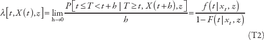
Let t denote analysis time (time since growth accelerated) and T denote duration (the length of a growth spell), a random variable. Thus t = 1 denotes the first year in a growth spell, t < 1 years prior to the beginning of the spell. X(t) is a vector of random variables that may influence the probability that a growth spell ends (also a random variable); x_t is the realization of X(t) at time t; and z is a vector of non-time-varying variables that may also have an impact on the length of a growth spell. z could contain realizations of X(t) before the beginning of a growth spell (i.e., x_t, t < 1) and also variables that have no time dimension at all (e.g., geographical variables). We want to estimate the effect of X(t) and z of interest on T.

Duration is usually modeled by parameterizing the hazard rate—the conditional probability that the spell will end in the next period—and estimating the relevant parameters using maximum likelihood. In the presence of both time-varying and time-invariant covariates, the hazard rate can be defined as (assuming continuous time):

where F(t|x_t,z) and f(t|x_t,z) are the c.d.f. and density function of T, respectively, conditioning on z and the realization of X at time t. The most popular approach to estimating equation (T2) is to assume a proportional hazard model—in effect, an assumption that the time dependence of λ, called the “baseline hazard,” is multiplicatively separable from its dependence on [X(t), z]—and to parameterize it by assuming that the relationship between λ and [X(t), z] is log–linear, and that the baseline hazard takes a particular functional form:

where λ₀(t) is assumed to obey a specific distribution whose parameters can be estimated along with the coefficient vector β. We have used as a baseline specification the assumption that λ₀(t) follows a Weibull distribution, that is, λ₀(t) = pt^p–1. The parameter p, which is estimated, determines whether duration dependence is positive (p > 1) or negative.

We start by characterizing the unconditional hazard rate, or the probability that a spell will end after a given number of years, conditional only on the fact that it has already lasted up to that point. We then examine the role of external shocks, then of institutions and variables related to social conflict (income distribution and ethnic heterogeneity), and then of a variety of other policy-related indicators, using some of the previous variables as controls. Results are presented in table T1 through table T4.

TABLE T1: Duration Regressions—Institutions

Model	Variable	Eight-year minimum spell		Five-year minimum spell
Model	Variable	Time ratio	p value	Time ratio	p value
1	Polity 2 (Polity IV database) Initial level	*1.12*	*0.10*	*1.10*	*0.01*
	Change within spell	*1.11*	*0.07*	*1.10*	*0.02*
	Spells/failures	46/17		66/35
2	Polity 2 (Polity IV database)	*1.12*	*0.04*	*1.12*	*0.00*
2	Spells/failures	51/17		72/37
3	Democracy (Polity IV database)	1.17	0.11	*1.22*	*0.00*
3	Spells/failures	51/17		72/37
4	Autocracy (Polity IV database)	*0.77*	*0.01*	*0.80*	*0.00*
4	Spells/failures	51/17		72/37
5	Executive recruitment (Polity IV database)	*1.42*	*0.02*	*1.35*	*0.00*
5	Spells/failures	51/17		72/37
6	Executive constraints (Polity IV database)	*1.35*	*0.07*	*1.42*	*0.00*
6	Spells/failures	51/17		72/37
7	Political competition (Polity IV database)	*1.26*	*0.05*	*1.23*	*0.00*
7	Spells/failures	51/17		72/37
8	Investment profile (ICRG)	1.64	0.29	*1.36*	*0.08*
8	Spells/failures	34/4		46/16

TABLE T2: Duration Regressions—Inequality and Fractionalization

Model	Variable	Eight-year minimum spell		Five-year minimum spell
Model	Variable	Time ratio	p value	Time ratio	p value
1	Inequality (Gini coefficient) Initial level	*0.87*	*0.02*	*0.85*	*0.00*
	Change within spell	1.08	0.31	0.94	0.28
	Spells/failures	22/6		32/14
2	Inequality (Gini coefficient)	*0.89*	*0.03*	*0.89*	*0.00*
2	Spells/failures	31/11		45/21
3	Ethnic fractionalization (Alesina, Spolaore, and Wacziarg 2005)	0.99	0.41	0.99	0.40
3	Spells/failures	56/19		86/45
4	Ethnic fractionalization (Alesina, Spolaore, and Wacziarg 2005)	*0.96*	*0.02*	*0.98*	*0.10*
	Inequality (Gini coefficient)	*0.91*	*0.03*	*0.89*	*0.00*
	Spells/failures	31/11		45/21

TABLE T3: Duration Regressions—Globalization

Model	Variable	Eight-year minimum spell		Five-year minimum spell
Model	Variable	Time ratio	p value	Time ratio	p value
1	Trade liberalization (Wacziarg–Welch dummy variable)
	Initial level	2.83	0.21	*6.56*	*0.00*
	Change within spell	*6.76*	*0.02*	*7.88*	*0.00*
	Spells/failures	38/16		61/33
2	Trade openness (based on PWT data, adjusted for structural characteristics)
	Initial level	*1.04*	*0.03*	1.01	0.33
	Change within spell	*1.04*	*0.01*	1.01	0.15
	Spells/failures	51/15		76/35
3	Financial integration (sum of external assets and liabilities)
	Initial level	1.01	0.54	1.00	0.87
	Change within spell	1.01	0.52	1.00	0.60
	Spells/failures	29/7		40/18
4	External debt liabilities
	Initial level	1.00	0.90	1.00	0.57
	Change within spell	1.00	0.92	1.00	0.18
	Spells/failures	29/7		40/18
5	FDI liabilities
	Initial level	1.00	0.99	1.03	0.27
	Change within spell	1.05	0.22	*1.11*	*0.02*
	Spells/failures	29/7		40/18

TABLE T4: Duration Regressions—Macroeconomic Volatility

Model	Variable	Eight-year minimum spell		Five-year minimum spell
Model	Variable	Time ratio	p value	Time ratio	p value
1	Log (1 + inflation)
	Initial level	1.00	0.94	1.01	0.58
	Change within spell	0.97	0.60	*0.99*	*0.02*
	Spells/failures	54/9		82/43
2	Log (1 + depreciation in the parallel exchange rate)
	Initial level	*0.94*	*0.02*	0.99	0.12
	Change within spell	*0.96*	*0.06*	*0.99*	*0.10*
	Spells/failures	23/9		34/18
3	Log (1 + moderate inflation)
	Initial level	0.96	0.45	*0.91*	0.0
	Change within spell	0.98	0.64	*0.94*	*0.02*
	Spells/failures	49/19		76/42
4	Average growth within spell	*0.84*	*0.01*	*0.86*	*0.00*
4	Spells/failures	57/19		88/46
5	Log (1 + inflation)
	Initial level	1.01	0.84	1.00	0.7
	Change within spell	0.98	060	*0.99*	*0.01*
	Average growth within spell	*0.81*	*0.01*	*0.86*	*0.00*
	Spells/failures	54/19		82/43
6	Log (1 + depreciation in the parallel exchange rate)
	Initial level	0.98	0.36	*0.99*	*0.06*
	Change within spell	*0.97*	*0.04*	*0.98*	*0.01*
	Average growth within spell	*0.64*	*0.00*	*0.85*	*0.00*
	Spells/failures	23/9		34/18
7	Debt/GDP change within spell
	Average growth within spell	0.97	0.20	*0.98*	*0.05*
	Log (1 + inflation)	*0.67*	*0.09*	*0.81*	*0.02*
	Initial level	1.01	0.88	1.00	0.93
	Change within spell	1.00	0.96	*0.99*	*0.02*
	Spells/failures	33/8		44/18

Figures 4.3, 4.4, 4.5, and 4.6

To assess the direct and indirect effect of reforms on the level of per capita GDP, we run separate regressions with growth and inequality as dependent variables. We include our different structural reform variables on the right-hand side (one variable at a time). All regressions use five-year averaged data.

To assess the direct effect of reforms and inequality on growth, we use standard dynamic (convergence) growth regressions of the form

where y_i,t is the log of per capita GDP of country i at time t,

is the average of the structural reform indicator between time t–4 and t,

is the level of inequality averaged between time t–4 and t, while

represents other controls also averaged between t–4 and t. Following Ostry, Berg, and Tsangarides (2014), in our baseline specification we include net inequality as a control variable. We do robustness checks in which the log of investment and the log of total education are also included as controls. A negative value for β₁ implies convergence. The coefficients of interest are γ₁, which captures the direct effect of reform on growth, and γ₂ which captures the effect of inequality on growth.

Analogous inequality convergence regressions are run to assess reforms’ effects on inequality. The equation is:

where Gini_i,t is the Gini coefficient for market inequality of country i at time t,

is the average of the structural reform indicator between time t-4 and t, while

represents other controls also averaged between t–4 and t. The coefficient of interest is γ₃, as this tells us the impact effect of reforms on inequality.

We include the averaged growth rate of per capita GDP as one of the Xs in the inequality regression to allow for two-way causation between inequality and growth. In this specification, reforms affect only the level of inequality in the steady state. However, the presence of lagged inequality on the right-hand side allows for dynamic effects, with reforms impacting the Gini gradually over time.

All regressions are estimated using system generalized method of moments (GMM) to try to account for reverse causality, endogeneity, and dynamic panel bias. Standard errors are clustered at the country level. While it is natural to use system GMM techniques to estimate dynamic panel regressions, we also checked for robustness by estimating pooled OLS as well as fixed-effect regressions. The results for the effects of reform on growth are similar irrespective of the estimation method. For the inequality regression, pooled OLS gives broadly similar results to system GMM while the results are usually weaker for fixed effects, suggesting that cross-country variation is important for identifying the reform–inequality relation.

Note that we include the contemporaneous level of the structural reform and other control variables on the right-hand side but instrument these with lags to account for potential endogeneity. Using the reform index at the beginning of the period instead of the contemporaneous average yields broadly similar results for the inequality regressions, although the effect of reforms on growth is somewhat weaker.

Tables T5 through T11 report the regression results for domestic finance, tariff reforms, current account liberalization, capital account liberalization, networks reforms, collective bargaining reforms, and law and order, respectively. In each table, column (1) reports the results for the whole sample (for figure 4.3); column (4) reports the results for the subsample of low-income countries (LICs) and middle-income countries (MICs) (for figure 4.4).

TABLE T5: Domestic Finance Reforms—Growth-Equity Trade-off

Variables	(1) Growth All Countries	(2) Growth All Countries	(3) Inequality All Countries	(4) Growth LIC and MIC	(5) Growth LIC and MIC	(6) Inequality LIC and MIC
Domestic finance	0.0630*** (0.0146)	0.0478*** (0.0149)	0.0065* (0.0038)	0.0633** (0.0261)	0.0210 (0.0263)	0.0137** (0.0058)
Net inequality	−0.1505*** (0.0527)	−0.0782* (0.0425)		−0.1940** (0.0911)	−0.0042 (0.0909)
Log (investment)		0.0410*** (0.0125)			0.0551*** (0.0089)
Log (education)		0.0004 (0.0085)			0.0143 (0.0171)
Lagged per capita GDP	−0.0126*** (0.0037)	−0.0129*** (0.0037)		−0.0130* (0.0072)	−0.0197** (0.0093)
Growth of per capita GDP			−0.0378 (0.0234)			−0.0128 (0.0402)
Lagged inequality			−0.0484*** (0.0147)			−0.0482 (0.0343)
Effect of reforms (75–50 percentile)	0.35	0.25	1.57	0.35	0.09	3.32
Observations	444	427	392	271	254	225
No. of countries	74	70	74	49	45	49
No. of instruments	65	63	65	36	63	37
AR2	0.237	0.344	0.230	0.0567	0.365	0.133
Hansen	0.450	0.393	0.319	0.310	0.988	0.234

Note: Details of reform variable in appendix 1. First column reports results of a standard growth regression (equation T4). Column 2 adds additional controls to the growth regression. Column 3 reports results for the dynamic inequality regression (equation T5) with change in market inequality on the LHS. Columns 4 to 6 repeat the same regressions but for the restricted sample of LICs and MICs only. Row “Effect of reforms” reports the effect on per capita GDP (in percent) and inequality (in Gini points) in the long run (30 years) of moving the reform index from the median to the seventy-fifth percentile. All regressions include country- and time-fixed effects. Estimation done using system GMM. P-value of Hansen and AR2 test reported. Robust standard errors clustered at country level in parentheses *** p < 0.01, ** p < 0.05, * p < 0.1.

Source: Data on per capita GDP growth and investment from Penn World Tables 7.1. Total education from Barro and Lee (2012). Net and market inequality from SWIID 5.0.

TABLE T6: Tariff Reforms—Growth-Equity Trade-off

Variables	(1) Growth All Countries	(2) Growth All Countries	(3) Inequality All Countries	(4) Growth LIC and MIC	(5) Growth LIC and MIC	(6) Inequality LIC and MIC
Tariff reform	0.0385** (0.0158)	0.0395** (0.0167)	0.0065* (0.0038)	0.0198 (0.0164)	0.0352* (0.0197)	0.0041 (0.0061)
Net inequality	−0.1311** (0.0536)	−0.1059*** (0.0394)		−0.0770* (0.0438)	−0.0492 (0.0422)
Log (investment)		0.0410*** (0.0071)			0.0265*** (0.0083)
Log (education)		−0.0063 (0.0087)			0.0163 (0.0110)
Lagged per capita GDP	−0.0052* (0.0027)	−0.0054* (0.0030)		−0.0012 (0.0036)	−0.0088** (0.0043)
Growth of per capita GDP			−0.0383* (0.0222)			−0.0040 (0.0177)
Lagged inequality			−0.0172 (0.0155)			−0.0271 (0.0169)
Effect of reforms (75–50 percentile)	0.15	0.16	0.19	NA	0.13	1.26
Observations	685	635	601	467	418	392
No. of countries	130	112	123	98	81	92
No. of instruments	81	97	89	89	81	89
AR2	0.262	0.876	0.997	0.166	0.491	0.849
Hansen	0.327	0.116	0.612	0.614	0.243	0.890

Notes: Data on per capita GDP growth and investment from Penn World Tables 7.1. Total education from Barro and Lee (2012). Net and market inequality from SWIID 5.0. Details of reform variable in appendix 1. First column reports results of a standard growth regression (equation T4). Column 2 adds additional controls to the growth regression. Column 3 reports results for the dynamic inequality regression (equation T5) with change in market inequality on the LHS. Columns 4 to 6 repeat the same regressions but for the restricted sample of LICs and MICs only. Row “Effect of reforms” reports the effect on per capita GDP (in percent) and inequality (in Gini points) in the long run (30 years) of moving the reform index from the median to the seventy-fifth percentile. All regressions include country- and time-fixed effects. Estimation done using system GMM. P-value of Hansen and AR2 test reported. Robust standard errors clustered at country level in parentheses. ***p < 0.01, **p < 0.05, p < 0.1

TABLE T7: Current Account Liberalization—Growth-Equity Trade-off

Variables	(1) Growth All Countries	(2) Growth All Countries	(3) Inequality All Countries	(4) Growth LIC and MIC	(5) Growth LIC and MIC	(6) Inequality LIC and MIC
Current account restrictions	0.0240* (0.0131)	0.0241** (0.0116)	0.0096** (0.0038)	−0.0020 (0.0140)	0.0095 (0.0150)	0.0095*** (0.0034)
Net inequality	−0.2075*** (0.0544)	−0.1144*** (0.0383)		−0.1181** (0.0538)	−0.0678 (0.0508)
Log (investment)		0.0337*** (0.0089)			0.0285*** (0.0094)
Log (education)		−0.0128** (0.0063)			−0.0035 (0.0138)
Lagged per capita GDP	−0.0082*** (0.0039)	−0.0070** (0.0027)		−0.0070 (0.0059)	−0.0081 (0.0067)
Growth of per capita GDP			−0.0299 (0.0251)			0.0169 (0.0296)
Lagged inequality			−0.0298* (0.0157)			−0.0382** (0.0194)
Effect of reforms (75–50 percentile)	0.12	0.12	2.83	−0.01	0.05	2.40
Observations	741	714	589	458	432	348
No. of countries	100	93	96	68	62	65
No. of instruments	71	103	57	61	101	55
AR2	0.110	0.196	0.980	0.134	0.195	0.580
Hansen	0.0524	0.644	0.641	0.334	0.988	0.788

Notes: Data on per capita GDP growth and investment from Penn World Tables 7.1. Total education from Barro and Lee (2012). Net and market inequality from SWIID 5.0. Details of reform variable in appendix 1. First column reports results of a standard growth regression (equation T4). Column 2 adds additional controls to the growth regression. Column 3 reports results for the dynamic inequality regression (equation T5) with change in market inequality on the LHS. Columns 4 to 6 repeat the same regressions but for the restricted sample of LICs and MICs only. Row “Effect of reforms” reports the effect on pc GDP (in percent) and inequality (in Gini points) in the long run (30 years) of moving the reform index from the median to the seventy-fifth percentile. All regressions include country- and time-fixed effects. Estimation done using system GMM. P-value of Hansen and AR2 test reported. Robust standard errors clustered at country level in parentheses. ***p < 0.01, **p < 0.05, p < 0.1

TABLE T8: Capital Account Liberalization—Growth-Equity Trade-off

Variables	(1) Growth All Countries	(2) Growth All Countries	(3) Inequality All Countries	(4) Growth LIC and MIC	(5) Growth LIC and MIC	(6) Inequality LIC and MIC
Capital account restrictions	0.0181 (0.0113)	0.0144 (0.0103)	0.0075** (0.0027)	−0.0001 (0.0098)	−0.0035 (0.0094)	0.0065** (0.0030)
Net inequality	−0.1957*** (0.0541)	−0.0979*** (0.0357)		−0.0988* (0.0591)	−0.0408 (0.0676)
Log (investment)		0.0348*** (0.0087)			0.0308** (0.0133)
Log (education)		−0.0064 (0.0069)			−0.0101 (0.0121)
Lagged per capita GDP	−0.0087*** (0.0037)	−0.0088*** (0.0029)		−0.0047 (0.0057)	−0.0057 (0.0051)
Growth of per capita GDP			−0.0271 (0.0229)			0.0232 (0.0239)
Lagged inequality			−0.0436*** (0.0159)			−0.0592*** (0.0202)
Effect of reforms (75–50 percentile)	0.20	0.16	3.84	0.00	−0.03	2.62
Observations	741	714	589	458	432	348
No. of countries	100	93	96	68	62	65
No. of instruments	61	103	57	61	101	55
AR2	0.135	0.214	0.804	0.140	0.204	0.743
Hansen	0.139	0.632	0.561	0.624	1	0.625

TABLE T9: Networks Reforms—Growth-Equity Trade-off

Variables	(1) Growth All Countries	(2) Growth All Countries	(3) Inequality All Countries	(4) Growth LIC and MIC	(5) Growth LIC and MIC	(6) Inequality LIC and MIC
Networks reform	0.0029 (0.0136)	0.0040 (0.0104)	0.0031 (0.0022)	−0.0121 (0.0126)	−0.0022 (0.0135)	0.0064** (0.0029)
Net inequality	−0.0473 (0.0723)	−0.0516 (0.0413)		−0.0839 (0.0618)	−0.0496 (0.0536)
Log (investment)		0.0389*** (0.0119)			0.0414** (0.0162)
Log (education)		−0.0063 (0.0076)			−0.0061 (0.0184)
Lagged per capita GDP	−0.0030 (0.0040)	−0.0047 (0.0047)		0.0074 (0.0081)	−0.0046 (0.0058)
Growth of per capita GDP			−0.0232 (0.0227)			0.0008 (0.0335)
Lagged inequality			−0.0407*** (0.0119)			−0.0444*** (0.0167)
Effect of reforms (75–50 percentile)	−0.03	0.06	2.22	−0.21	−0.03	4.31
Observations	561	534	431	344	318	248
No. of countries	86	76	80	60	51	55
No. of instruments	85	89	48	45	83	42
AR2	0.180	0.234	0.624	0.127	0.203	0.138
Hansen	0.565	0.786	0.977	0.937	1	0.642

TABLE T10: Collective Bargaining Reforms—Growth-Equity Trade-off

Variables	(1) Growth All Countries	(2) Growth All Countries	(3) Inequality All Countries	(4) Growth LIC and MIC	(5) Growth LIC and MIC	(6) Inequality LIC and MIC
Current account restrictions	0.0404 (0.0249)	0.0118 (0.0250)	0.0027 (0.0060)	−0.0331 (0.0464)	−0.0011 (0.0396)	0.0116* (0.0063)
Net inequality	−0.0775 (0.0769)	−0.0563 (0.0370)		−0.0292 (0.1173)	0.0428 (0.0873)
Log (investment)		0.0463*** (0.0135)			0.0275* (0.0166)
Log (education)		0.0102 (0.0172)			−0.0027 (0.0453)
Lagged per capita GDP	−0.0040 (0.0044)	−0.0076 (0.0052)		−0.0124* (0.0074)	−0.0010 (0.0143)
Growth of per capita GDP			−0.0532* (0.0306)			−0.0344 (0.0320)
Lagged inequality			−0.0542*** (0.0149)			−0.0349** (0.0158)
Effect of reforms (75–50 percentile)	0.24	0.06	0.54	0.15	−0.01	3.19
Observations	451	439	431	220	208	212
No. of countries	96	90	95	66	60	65
No. of instruments	81	81	82	64	80	67
AR2	0.353	0.516	0.932	0.239	0.235	0.677
Hansen	0.717	0.733	0.926	0.996	1	1

Notes: Data on per capita GDP growth and investment from Penn World Tables 7.1. Total education from Barro and Lee (2012). Net and market inequality from SWIID 5.0. Details of reform variable in appendix 1. First column reports results of a standard growth regression (equation T4). Column 2 adds additional controls to the growth regression. Column 3 reports results for the dynamic inequality regression (equation T5) with change in market inequality on the LHS. Columns 4 to 6 repeat the same regressions but for the restricted sample of LICs and MICs only. Row “Effect of reforms” reports the effect on pc GDP (in percent) and inequality (in Gini points) in the long run (30 years) of moving the reform index from the median to the seventy-fifth percentile. All regressions include country- and time-fixed effects. Estimation done using system GMM. P-value of Hansen and AR2 test reported. Robust standard errors clustered at country level in parentheses. ***p < 0.01, **p < 0.05, p < 0.1

TABLE T11: Law and Order—Growth-Equity Trade-off

Variables	(1) Growth All Countries	(2) Growth All Countries	(3) Inequality All Countries	(4) Growth LIC and MIC	(5) Growth LIC and MIC	(6) Inequality LIC and MIC
Law and order (ICRG)	0.0474** (0.0225)	0.0344 (0.0220)	0.0043 (0.0043)	0.0622*** (0.0215)	0.0462** (0.0185)	0.0023 (0.0067)
Net inequality	−0.0918 (0.0988)	−0.0616 (0.0480)		0.0187 (0.1021)	−0.0143 (0.0455)
Log (investment)		0.0135* (0.0077)			0.0157** (0.0065)
Log (education)		−0.0181 (0.0115)			0.0110 (0.0112)
Lagged per capita GDP	−0.0080*** (0.0025)	−0.0136*** (0.0034)		−0.0033 (0.0042)	−0.0078 (0.0048)
Growth of per capita GDP			−0.0761*** (0.0261)			−0.0114 (0.0404)
Lagged inequality			−0.0340** (0.0170)			−0.0232 (0.0164)
Effect of reforms (75–50 percentile)	0.39	0.23	1.73	0.61	0.38	1.14
Observations	471	435	426	324	289	283
No. of countries	108	97	104	77	67	74
No. of instruments	43	79	43	43	79	43
AR2	0.990	0.675	0.286	0.995	0.448	0.872
Hansen	0.0216	0.134	0.593	0.568	0.818	0.334

TOTAL EFFECT

As discussed in the text, and shown in the tables, for a number of indicators we find that reforms increase inequality as well as growth. In chapter 3, we showed that higher levels of inequality may reduce growth. This raises the question: what is the total effect of reforms on growth? That is, after taking into account the higher inequality following reforms, how much lower is the effect of reforms on growth (and is it even positive)? To answer this question, we carry out some simple calculations by combining results from the separate growth and inequality regressions. First, consider the direct effect of reforms on the steady-state level of log of per capita GDP (holding inequality constant). From equation (T4), a change in the reform index from the median to the seventy-fifth percentile, denoted by ΔSR, results in a steady-state increase in log of per capita GDP of

. Now, the same increase in the reform index leads to a steady-state increase in the Gini coefficient of

(from equation T5). The indirect effect of this increase in inequality on per capita GDP (in steady state) is therefore given by

, where γ₂ is the coefficient on inequality in the growth regression. Finally, the total effect on growth is the sum of direct and indirect effects. Figure 4.5 reports results for this calculation.

Figures 5.3, 5.4, and 5.5

To assess the impact of capital account liberalization, we follow the autoregressive distributed lag approach of Romer and Romer (2004), among others. This approach is particularly suited to assess the dynamic response of the variable of interest in the aftermath of a reform (a capital account liberalization episode in our case). The methodology consists of estimating a univariate autoregressive equation and deriving the associated impulse response functions:

where g is the annual change in the log of output (or the Gini coefficient, or the labor share); D is a dummy variable that is equal to 1 at the start of a capital account liberalization episode and zero otherwise; a_i are country-fixed effects included to control for unobserved cross-country heterogeneity; γ_t are time-fixed effects to control for global shocks. We include lagged output growth (inequality) to control for the normal dynamics of output (inequality). In addition, because the variables affecting output (inequality) in the short term are typically serially correlated, this also helps to control for various factors that may influence output (inequality).

Finally, because several types of economic reforms are often implemented simultaneously—this is particularly the case for current account and capital account reforms—we include in the baseline a set of other structural reform variables (X) to distinguish the effect of capital account liberalization episodes from others. Specifically, the set of reform variables included as controls are (1) current account reforms, defined as an episode where the annual change of the Quinn and Toyoda (2008) measure of current account openness exceeds by two standard deviations the average annual change over all observations, and (2) regulation reforms, defined as an episode where the annual change in a composite measure of credit, product, and labor market regulation exceeds by two standard deviations the average annual change over all observations.

Equation (T6) is estimated using OLS on an unbalanced panel of annual observations from 1970 to 2010 for 149 advanced and developing economies. While the presence of a lagged dependent variable and country-fixed effects may in principle bias the estimation of δ_j and β_j in small samples, the length of the time dimension mitigates this concern. The finite sample bias is in the order of 1/T, where T in our sample is 41. Robustness checks using a two-step system-GMM estimator confirm the validity of the results. The number of lags chosen is two, but different lag lengths are tested as a robustness check.

Impulse response functions are used to describe the response of growth and inequality following a capital account liberalization episode. The shape of these response functions depends on the value of the δ and β coefficients. For instance, the simultaneous response is δ₀, the one-year-ahead cumulative response is δ₀(δ₁ + β₀δ₀). The confidence bands associated with the estimated impulse-response functions are obtained using the estimated standard errors of the estimated coefficients, based on clustered (at country-level) heteroskedasticity robust standard errors.

Figure 5.3 shows the impulse-response functions for growth and the Gini measure of inequality, figure 5.4 for the top income shares, and figure 5.5 for the labor share.

Figures 5.6 and 5.8

It is commonly argued that there are certain threshold levels of financial development (in particular the depth of the credit market) that an economy needs to attain before it can benefit from, and reduce the risks associated with, financial globalization. Capital account liberalization may allow better consumption smoothing and lower volatility for countries with strong financial institutions, but where institutions are weak and the access to credit is not inclusive, it may have limited output gains and further exacerbate inequality by increasing the bias in financial access in favor of people who are well off.

We re-examine this hypothesis by assessing whether the effect of capital account liberalization depends on the strength of financial institutions—depth and access to credit—and whether liberalization episodes are followed by crises. Specifically, we estimate the following equation:

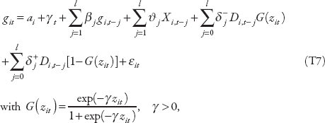
in which z is an indicator of financial development, normalized to have zero mean and unit variance, and G(z_it) is the corresponding smooth transition function of the degree of financial development—in the case of crises the G(.) function takes value one if episodes are followed by crises, zero otherwise. This approach is equivalent to the smooth transition autoregressive (STAR) model to assess nonlinear effects above/below a given threshold or regime. The main advantage of this approach relative to estimating structural vector autoregressive models for each regime is that it uses a larger number of observations to compute the impulse-response functions of only the dependent variables of interest, improving the stability and precision of the estimates. This estimation strategy can also more easily handle the potential correlation of the standard errors within countries, by clustering at the country level.

Figure 5.6 shows how the impact of capital account liberalization on growth and inequality depends on financial depth and inclusion and on the occurrence of crisis. Figure 5.8 shows how the impact on inequality depends on financial depth and inclusion in the case of LICs.

Figures 6.3, 6.4, and 6.5

To assess the distributional impact of fiscal consolidation episodes over the short and medium term, the paper follows the method proposed by Jordà (2005), which consists of estimating the dynamic change in inequality in the aftermath of fiscal adjustment episodes. Specifically, for each future year k the following equation has been estimated on annual data:

with k = 1...8, where G represents our measure of inequality (proxied by the Gini coefficient for disposable income); D_i,t is a dummy variable that takes the value equal to 1 for the starting date of a consolidation episode in country i at time t and 0 otherwise;

are country-fixed effects;

is a time trend; and β_k measures the impact of fiscal consolidation episodes on the change of the Gini coefficient for each future period k. Because fixed effects are included in the regression, the dynamic impact of consolidation episodes should be interpreted as changes in the Gini coefficient compared to a baseline country-specific trend.

Equation (T7) is estimated using the panel-corrected standard error (PCSE) estimator. This procedure is better placed to deal with the nature of our data (such as a small number of countries compared to the number of years) and to correct for panel-specific heteroskedasticity and serial correlation. The number of lags (l) has been chosen to be equal to 2, as this produces the best specification, but the results are extremely robust to different numbers of lags included in the specification (see robustness checks presented in the next section).

The dynamic responses of inequality to fiscal adjustments are then obtained by plotting the estimated β_k for k = 0, 1...8, with confidence bands for the estimated effects being computed using the standard deviations associated with the estimated coefficients β_k. While the presence of a lagged dependent variable and country-fixed effects may in principle bias the estimation of

and β_k in small samples, the length of the time dimension mitigates this concern. The finite sample bias is in the order of 1/T, where T (total number of time periods) in our sample is 32.

Figure 6.3 shows the response of inequality to fiscal consolidation using the method described above. To assess the effects of fiscal consolidation on the distribution of income between various groups, equation (T7) is also estimated for wage and profit income (figure 6.4), and for short-term and long-term unemployment (figure 6.5).

Figure 7.1

To measure monetary policy shocks, we adapt the approach developed by Auerbach and Gorodnichenko (2013) to identify fiscal policy shocks. We proceed in two steps. First, using forecasts from Consensus Economics, we compute unexpected changes in policy rates (proxied by short-term rates) using the forecast error of the policy (short-term) rates (

)—defined as the difference between the actual policy short-term rates at the end of the year (

) and the rate expected by analysts as of the beginning of October for the end of the same year (

We then regress for each country the forecast errors of the policy rates (

) on similarly computed forecast errors of inflation (FE^inf) and output growth (FE^g):

where

is the difference between the CPI inflation (GDP growth) at the end of the year and the inflation (GDP growth) expected by analysts as of the beginning of October for the end of the same year; the residuals—∈_i,t—capture exogenous monetary policy shocks. Monetary policy shocks are identified for each country covered in Consensus Economics.

This methodology overcomes two problems that may otherwise confound the causal estimation of the effect of monetary policy shocks on inequality. First, using forecast errors eliminates the problem of “policy foresight,” namely that people may receive news about changes in monetary policy in advance and may alter their consumption and investment behavior well before the changes in policy occur. An econometrician who uses just the information contained in the change in actual policy rate would be relying on a smaller information set than that used by economic agents, leading to inconsistent estimates of the effects of monetary policy shocks. In contrast, by using forecast errors in policy rates, this methodology effectively aligns the economic agents’ and the econometrician’s information sets. Second, by purging news (that is, unexpected changes) in growth and inflation from the forecast errors in the short-term rate we significantly reduce the likelihood that the estimates capture the potentially endogenous response of monetary policy to changes in growth or inflation.

Figure 7.1 illustrates the measure of monetary policy shocks using our method for the United States and shows that it is quite similar to the popular measure of Romer and Romer (2004).

Figures 7.2, 7.3, 7.4, and 7.5

To estimate the impact of monetary policy shocks on inequality in the short and medium term, we follow the method proposed by Jordà (2005) discussed earlier, which consists of estimating impulse-response functions directly from local projections. Specifically, for each future period k the following equation is estimated on annual data:

where y is the (log) of net income inequality; MP_i,t are exogenous monetary policy shocks; α_i are country-fixed effects included to control for unobserved cross-country heterogeneity of inequality and also to control for the fact that in some countries inequality is measured using income data while in other countries using consumption data; ϑ_t are time-fixed effects to control for global shocks; X is a set of controls including lagged monetary policy shocks and lagged changes in inequality.

The baseline analysis focuses on net rather than gross income for two reasons. First, the source of data (the Luxembourg Income Study) through which gross market Gini data are computed in the SWIID dataset is based on household disposable income, and therefore is likely to be less subject to measurement errors. Second, we want to capture the overall effects of monetary policy shocks on inequality including through effects on redistribution (that is, tax and transfers). That said, the results based on market income are robust and not statistically different from those based on net income.

Equation (T10) is estimated for k=0, …, 4—that is, up to five years after the shock. Impulse-response functions are computed using the estimated coefficients β^k and the confidence intervals using the estimated standard errors of these coefficients. The sample period—determined by the availability of the series of monetary policy shocks and inequality—is from 1990 to 2013. The estimates for 32 advanced economies and emerging-market countries are based on clustered robust standard errors.

Figure 7.2 shows that our monetary policy shocks have the expected effects on macroeconomic variables such as output, inflation, and asset prices. The figures that follow show the impact of monetary policy shocks on the Gini measure of inequality (figure 7.3), the share of wage income (figure 7.4), and top income shares (figure 7.5).