General Topology

In this section we prove four lemmas, all part of a program to construct real-valued continuous functions on topological spaces. For the moment we are concerned with a rather special sort of topological space. A space is normal * iff for each disjoint pair of closed sets, A and B, there are disjoint open sets U and V such that A ⊂ U and B ⊂ V. A T₄-space is a normal space which is T₁ ({x} is closed for each x). If it is agreed that a set U is a neighborhood of a set A iff A is a subset of the interior U⁰ of U, then the definition of normality can be stated: a space is normal iff disjoint closed sets have disjoint neighborhoods. There is another restatement of the condition which is also suggestive. A family of neighborhoods of a set is a base for the neighborhood system of the set iff every neighborhood of the set contains a member of the family. If W is a neighborhood of a closed subset A of a normal space X, then there are disjoint open sets U and V such that A ⊂ U and X ~ W⁰ ⊂ V, and hence the arbitrary neighborhood W of A contains the closed neighborhood U^–. Consequently the family of closed neighborhoods of a closed set A is a base for the neighborhood system of A if the space is normal. The converse is also true, for if A and B are disjoint closed sets and W is a closed neighborhood of A which is contained in X ~ B, then W⁰ and X ~ W are disjoint open neighborhoods of A and B respectively.

There is a condition which for T₁-spaces is intermediate to Hausdorff and normal, and under certain circumstances implies normality. A topological space is regular iff for each point x and each neighborhood U of x there is a closed neighborhood V of x such that V ⊂ U; that is, the family of closed neighborhoods of each point is a base for the neighborhood system of the point. An equivalent statement: for each point x and each closed set A, if

, then there are disjoint open sets U and V such that x ε U and A ⊂ V regular space which is also T₁ is called a T₃-space. Recall that a Lindelöf space is a topological space such that each open cover has a countable subcover.

PROOF Suppose A and B are closed disjoint subsets of X. Because X is regular, for each point of A there is a neighborhood whose closure fails to intersect B and consequently the family at of all open sets whose closures do not intersect B is a cover of A. Similarly, the family

of all open sets whose closures do not intersect A is a cover of B, and

is a cover of X. There is then a sequence {U_n, n ε ω} of members of

which covers A, and a sequence {V_n, n ε ω} of members of

which covers B. Let

and let

since U_n′ ∩ V_m is void for m

n, it follows that U_n′ ∩ V_m′ is void for m

n. Applying the same argument with the roles of U and V interchanged, U_n′ ∩ V_m′ is void for all m and n and consequently

is disjoint from

. Finally, V_p^– ∩ A and U_p^– ∩ B are void for all p and hence the open disjoint sets

and

contain A and B respectively.

In particular, a regular topological space satisfying the second axiom of countability is always normal.

PROOF The map e followed by projection P_f into the f-th coordinate space is continuous because P_f ∘ e(x) =f(x). Consequently, by theorem 3.3, e is continuous. To prove statement (b) it is sufficient to show that the image under e of an open neighborhood U of a point x contains the intersection of e[X] and a neighborhood of e(x) in the product. Choose a member f of F such that f(x) does not belong to the closure of f[X ~ U]. The set of all y in the product such that

is open, and evidently its intersection with e[X] is a subset of e[U]. Hence e is an open map of X onto e[X]. Statement (c) is clear.

The preceding lemma reduces the problem of embedding a space topologically in a cube to the problem of finding a “rich” set of continuous real-valued functions on the space. There are topological spaces on which each continuous real-valued function is constant. For example, any indiscrete space has this property. There are less trivial examples; there are regular Hausdorff spaces on which every real continuous function is constant.* A topological space X is called completely regular iff for each member x of X and each neighborhood U of x there is a continuous function f on X to the closed unit interval such that f(x) = 0 and f is identically one on X ~ U. It is clear that the family of all continuous functions on a completely regular space to the unit interval [0,1] distinguishes points and closed sets, in the sense of the preceding lemma. (The converse statement is also true, but will not be needed here.) If a completely regular space is T₁ ({x} is closed for each x), then the family of continuous functions on the space to [0,1] also distinguishes points. A completely regular T₁-space is called a Tychonoff space. If X is a Tychonoff space and F is the family of all continuous functions on X to [0,1], then the embedding lemma 4.5 shows that the evaluation map of X into the cube Q^F is a homeomorphism. Thus each Tychonoff space is homeomorphic to a subspace of a cube. This fact is actually characteristic of Tychonoff spaces, as will presently be demonstrated.

Each normal T₁-space is a Tychonoff space in view of Urysohn’s lemma 4.4. Each completely regular space is regular, for if U is a neighborhood of x and f is a continuous function which is zero at x and one on X ~ U, then V = {y: f(y) < ½} is an open set whose closure is contained in {y: f(y)

½}, which is a subset of U. For T₁-spaces there is a hierarchy of so-called separation axioms: Hausdorff, regular, completely regular, and normal. Except for normality, these properties are hereditary, in the sense that each subspace of a space X enjoys the property if X does. The product of spaces of each of these types is again of the same type, excepting, again, normality. The proofs of these facts are left as problems (4.H) except for the following, which is needed now.

There are many topological spaces in which the topology is derived from a notion of distance. A metric for a set X is a function d on the cartesian product X × X to the non-negative reals such that for all points x, y, and z of X,

It is easy to describe the class of topological spaces to which the foregoing metrization theorem applies.

The metrization theorem for spaces which are not necessarily separable depends heavily on the ideas which we have already exploited. A brief discussion of methodology will indicate where the procedure used so far can be improved. The construction of a metric for X is accomplished by finding a family of mappings of X into pseudo-metrizable spaces. But observe: so far the only space which has been used as the range space is the unit interval Q. Stated in slightly different form, if f is a function on X to Q, then one may construct a pseudo-metric for X by letting d(x,y) ⁼ | f(x) – f(y) |. The Urysohn metrization is accomplished by using a countable number of pseudo-metrics of this sort, and the problem is to generalize this construction. If F is a family of functions on X to Q, then a possible candidate for a pseudo-metric is the sum : ∑ {| f(x) – f(y) | : f ε F}. This sum must be continuous in x and y in order that the identity map of X into the pseudo-metric space (X,d) be continuous, and a condition much weaker than finiteness of the family F will ensure continuity. It is sufficient, to obtain continuity, that for each point x of X there be a neighborhood U of x such that all but a finite number of the members of F vanish on U; in other words, a sort of local finiteness suffices. This notion of local finiteness is the key to the problem.

21 THEOREM Each open cover of a pseudo-metrizable space has an open σ-discrete refinement.

PROOF Let

be an open cover of the pseudo-metric space (X,d). The first step in the proof is the decomposition of each member U of

into “concentric disks.” For each positive integer n and each member U of

let U_n be the set of all members x of U such that dist [x,X ~ U]

2^–ⁿ. Because of the triangle inequality it is clear that dist [U_n,X ~ U_n₊₁]

2^–ⁿ – 2^–ⁿ^–1 = 2^–ⁿ^–1. Choose a relation < which well orders the family

(see 0.25h) and for each positive integer n and each member U of

let

and V < U}. For each U and V in

and each positive integer n it is true that U_n* ⊂ X ~ V_n₊₁, or V_n* ⊂ X ~ U_n₊₁, depending on whether U follows or precedes V in the ordering. In either case dist [U_n*,V_n*]

2^–ⁿ^–1. It follows that if U_n^~ is defined to be the set of all points x such that the distance from x to U_n* is less than 2^–ⁿ^–3, then dist [U_n^~,V_n^~]

2^–ⁿ^–2 and hence for each fixed n the family of all sets of the form U_n^~ is discrete. Let

be the family of U_n^~ for all n and all U in

. Then

is an open cover of X, for if U is the first member of

to which x belongs, then surely x ε U_n^~ for some n. Evidently U_n^~ ⊂ U, and consequently

is a σ-discrete open refinement of

22 Notes There are really two metrization problems. The topological problem has just been treated and the problem of uniform metrization will be considered in chapter 7 (statement and history are given there). Curiously enough a satisfactory solution of the latter was found much earlier than a solution of the former. Urysohn’s theorem, although treating only a special case, was certainly the most satisfactory theorem of the topological sort until very recently. The key to the present reasonably satisfactory situation was furnished by two papers. Dieudonné [1] initiated a study of spaces with the property that each open cover has an open locally finite refinement (paracompact spaces; see chapter 5). A. H. Stone [1] showed that each metrizable space is paracompact (a special case of this theorem was earlier demonstrated by C. H. Dowker [1]). The σ-locally finite characterization was then discovered independently, by Nagata [1] and by Smirnov [1]. The σ-discrete characterization is due to Bing [1]. The proof of necessity (4.21) of the metrizability conditions is actually an initial fragment of Stone’s proof of paracompactness.

Smirnov [2] has also showed that paracompactness together with local metrizability implies metrizability.

Finally a brief statement of the role of pseudo-metrizable spaces might be made. Most of the spaces which occur naturally in analysis are pseudo-metric rather than metric, and even in the metrization problem a construction via pseudo-metrics was convenient. Of course, one may always replace a pseudo-metric space by a related metric space (theorem 4.15), but the process of taking quotient spaces becomes a bit tedious and for most purposes the requirement d(x,y) = 0 iff x = y is completely irrelevant. One is tempted to work exclusively with pseudo-metrics, but this has disadvantages, for example, when one seeks to construct a topological map. A possible way out is to redefine “topological map” to mean a relation which induces a one-to-one intersection and union-preserving map on the topologies.

AREGULAR SPACES

(a) Let X be a regular space and let be the family of all subsets of the form {x}^– for x in X. Then is a decomposition of X, the projection of X onto the quotient space is both open and closed, and the quotient space is regular Hausdorff. (If A is a subset of X which is either open or closed, then {x}^– ⊂ A whenever x ε A.)

(b) The product of regular spaces is again regular.

BCONTINUITY OF FUNCTIONS ON A METRIC SPACE

A function f on a pseudo-metric space (X,d) to a pseudo-metric space (Y,e) is continuous iff for each x in X and each > 0 there is δ > 0 such that e(f(x), f(y)) < if d(x,y) < δ.

CPROBLEM ON METRICS

Let f be a continuous real-valued function defined on the set of all non-negative real numbers, such that f(x) = 0 iff x = 0, f is non-decreasing, and f(x+y) f(x) + f(y) for all non-negative numbers x and y. (A function satisfying this last condition is called subadditive.) If (X,d) is a metric space and e(x,y) = f(d(x,y)), then (X,e) is a metric space, and the metric topology of the space (X,e) is identical with that of (X,d). (A particular case of this result which occurs frequently in the literature: f(x) = x/(1 + x).)

DHAUSDORFF METRIC FOR SUBSETS

Let (X,d) be a metric space of finite diameter, and let be the family of all closed subsets. For r > 0 and A in let V_r(A) = {x: dist (x,A) < r}, and define, for members A and B of , d′(A,B) = inf {r: A ⊂ V_r(B) and B ⊂ V_r(A)}. d′ is the Hausdorff metric; it is not the same as the distance between sets used in the text.

(a) (, d′) is a metric space, and the map which carries x in X into {x} in is an isometry of X onto a subspace of .

(b) The topology of the Hausdorff metric for is not determined by the metric topology for X. For example, let X be the set of all positive real numbers, let d(x,y) = | x/(1 + x) –y/(1 +y)|, and let e(x,y) = min [1,| x – y |]. Then the metric topologies of (X,d) and (X,e) are identical, but those of (, d′) and (,e′) are different. (In (, d′) the set of all positive integers is an accumulation point of the family of all its finite subsets.)

Note For information and references on this topic see Michael [2].

EEXAMPLE (THE ORDINALS) ON THE PRODUCT OF NORMAL SPACES

The product of normal spaces is not generally normal.* Let Ω₀ be the set of all ordinal numbers less than the first uncountable ordinal Ω and let Ω′ be Ω₀ ∪ {Ω} each with the order topology.

(a) Interlacing lemma Let {x_n, n ε ω} and {y_n, n ε ω} be two sequences in Ω₀ such that x_n y_n x_n₊₁ for each n. Then both sequences converge, and to the same point of Ω_0.

(b) If A and B are closed disjoint subsets of Ω₀, then Ω, is not an accumulation point of both A and B.

(c) Both Ω₀ and Ω′ are normal. (If A and B are closed disjoint subsets and the first point of A ∪ B belongs to A, find a finite sequence a₀, b₀, a₁, … a_n (or b_n) such that a_i ε A, b_i ε B, no point of A is between a_i and b_i, and no point of B is between b_i and a_i₊₁, for each i. The intervals (a_i,b_i] are both open and closed.)

(d) If f is a function on Ω₀ to Ω₀ such that f(x) x for each x, then for some x in Ω₀ the point (x,x) is an accumulation point of the graph of f. (Define a sequence, inductively, such that x_n₊₁ = f(x_n), observe that x_n f(x_n) x_n₊₁, and use the interlacing lemma.)

(e) The product Ω₀ × Ω′ is not normal. (Let A be the set of all points (x,x), and let B = Ω₀ × {Ω}. If U is a neighborhood of A let f(x) be the smallest ordinal larger than x such that . Then (d) applies.)

FEXAMPLE (THE TYCH0N0FF PLANK) ON SUBSPACES OF NORMAL SPACES

A subspace of a normal space may fail to be normal. Let Ω′ be the set of ordinal numbers not greater than the first uncountable ordinal Ω, and let ω′ be the set of ordinals not greater than the first infinite ordinal, ω, each with the order topology. The product Ω′ × ω′ is called the Tychonoff plank. It is not difficult to prove directly that the plank is normal; however, this fact is an immediate consequence of a theorem of the next chapter. Let X be (Ω′ × ω′) ~ {(Ω,ω)}, so that X is the plank with a corner point removed. Let A be the set of all points of X with first coordinate Ω and let B be the set of all points with second coordinate ω. Then there are no disjoint neighborhoods of A and B. (If U is a neighborhood of A, then for x in ω let f(x) be the first ordinal such that if y > f(x), then (y,x) ε U. The supremum of the values of f is less than Ω.)

GEXAMPLE: PRODUCTS OF QUOTIENTS AND NON-REGULAR HAUSDORFF SPACES

Let X be a regular Hausdorff space which is not normal, and let A and B be disjoint closed sets such that each neighborhood of A intersects each neighborhood of B. Let Δ be the set of all (x,x) for x in X (Δ is the identity relation on X).

(a) Let R = Δ ∪ (A × A). Then R is closed in X × X and the quotient space X/R is a Hausdorff space which is not regular. (The members of the quotient space are A, and {x} for x in X ~ A.)

(b) Let S = Δ ∪ (A × A) ∪ (B × B). Then S is closed in X × X, but X/S is not a Hausdorff space. (The members of X/S are A, B, and {x} for each x in X ~ {A ∪ B).)

(c) There is a natural map of X × X onto (X/S) × (X/S) which carries (x,y) into (S[x],S[y]). It is natural to ask whether this map is open, provided X/S is given the quotient topology and (X/S) × (X/S) and X × X are given the product topologies. (This is equivalent to asking whether the product of quotients is topologically equivalent to the quotient of the product.) If S is the relation defined in (b), then the map is not open. (Consider the neighborhood X × X ~ (A × A ∪ B × B ∪ Δ) of A × B.)

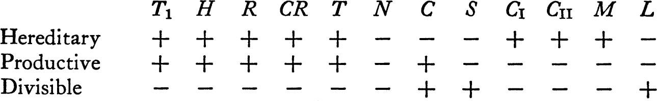
HHEREDITARY, PRODUCTIVE, AND DIVISIBLE PROPERTIES

A property P of a space is hereditary iff each subspace of a space with P also has P; it is productive iff the product of spaces enjoying P has P; and it is divisible iff the quotient space of each space with P has P. Consider the properties: T₁, H = Hausdorff, R = regular, CR = completely regular, T = Tychonoff, N = normal, C = connected, S = separable, C_I = first axiom of countability, C_II = second countability axiom, M = metrizable, and L = Lindelöf. The following table is filled out + or –, depending on whether the property at the head of the column is or is not of the sort listed on the left. Show by example (most of the necessary examples have already been mentioned in the problems) or proof that the listing is correct.

Quite different results are obtained if one varies the problem by considering only closed subspaces, or only open maps.

IHALF-OPEN INTERVAL SPACE

Let X be the set of all real numbers with the half-open interval topology (a base is the family of all half-open intervals [a,b); see 1.K and 1.L). Then:

(a) X is regular.

(b) X is normal. (Recall that every open cover of X has a countable subcover.)

(c) The product space X × X is not normal. (Let Y = {(x,y) : x + y = 1}, let A be the set of all members of Y with first coordinate irrational, and let B = Y ~ A. Assume that U and V are disjoint neighborhoods of A and B, and for x in A let f(x) = sup {e: [x,e) × [1 – x,e) ⊂ U}. Then f is a function on the set of all irrational numbers and f is never zero. The contradiction depends on the fact that for some positive integer n there is a rational number which is an accumulation point of {x: f(x) 1/n}. This fact is an immediate consequence of the theorem that the space of real numbers (with the usual topology) is of the second category (see chapter 7), but a direct proof seems awkward.)

Note This example is due to Sorgenfrey [1].

JTHE SET OF ZEROS OF A REAL CONTINUOUS FUNCTION

A subset of a topological space is called a G_δ iff it is the intersection of the members of a countable family of open sets.

(a) If f is a continuous real valued function on X, then f^–1[0] is a G_δ. (The set {0} is a G_δ in the space of all real numbers.)

(b) If A is a closed G_δ in a normal topological space X, then there exists a continuous real-valued function f such that A = f^–1[0].

KPERFECTLY NORMAL SPACES

A topological space is called perfectly normal iff it is normal and each closed subset is a G_δ.

(a) Each pseudo-metrizable space is perfectly normal.

(b) The product of an uncountable number of unit intervals is not perfectly normal. (A G_δ in such a space cannot consist of a single point.)

LCHARACTERIZATION OF COMPLETELY REGULAR SPACES

A topological space is completely regular iff it is homeomorphic to a subspace of a product of pseudo-metric spaces.

MUPPER SEMI-CONTINUOUS DECOMPOSITION OF A NORMAL SPACE

The image of a normal topological space under a closed continuous map is a normal space.

* This nomenclature is an excellent example of the time-honored custom of referring to a problem we cannot handle as abnormal, irregular, improper, degenerate, inadmissible, and otherwise undesirable. A brief discussion of the abnormalities of the class of normal spaces occurs in the problems at the end of the chapter.

* It is possible to do part of this problem a little more efficiently using methods from the following chapter. However, the facts given here will be useful later. I believe the example is due to J. Dieudonné and A. P. Morse, independently.