Kenneth M. Johnson
This chapter describes where rural America is and how the population of rural America is changing. Rural America is large and diverse. Some rural areas are growing rapidly, whereas other rural communities house far fewer people today than they did a century ago. Rural concerns are often overlooked in a nation dominated by urban interests. Yet a vibrant rural America contributes to the nation’s intellectual and cultural diversity and provides most of the nation’s food, minerals, clean air, and clean water. The demographic change in rural America has implications for poverty and family well-being. This chapter considers the unfolding demographic story of rural America, setting the stage for the remainder of the book. It examines how poverty influences the viability of rural communities, the lives of rural residents, and the contributions rural America makes to the nation’s material, environmental, and social well-being.
Rural America is a simple term describing a remarkably diverse collection of people and places. More than 50 million people live rurally, and these areas cover nearly 75 percent of the United States. Rural America spans a broad spectrum of landscapes that includes some of the best farmland in the world. It spreads across the vast agricultural heartland of the Great Plains and Corn Belt and extends from the Canadian border deep into Texas. Rural America holds the highly productive fruit and vegetable regions of California, Florida, and the Southwest, as well as dairy regions in Wisconsin, upstate New York, and New England. But there is far more to rural America than agriculture. It includes sprawling exurban areas on the outer edges of the nation’s largest metropolitan areas; the vast arid range and desert lands in the Southwest; the deep, mountainous forests of the Pacific Northwest; the flat and humid coastal plain of the Southeast; the hardscrabble towns and hollows of the Appalachians; the rocky shorelines and working forests of New England, where rural villages look much as they did a hundred years ago; and the glaciers and fjords of Alaska.
Rural economies also depend on more than just agriculture. Some rely on auto supplier plants strung along the interstates of the auto corridor from the Great Lakes to Tennessee. Elsewhere, coal, ore, oil, and gas are extracted, processed, and shipped through a complex network of pipelines, barges, ships, and railroads to urban consumers hundreds or thousands of miles away. Warehouses and distribution centers clustered around major rural interstate interchanges facilitate the movement of goods and products. In other rural regions, struggling industrial towns facing intense global competition try to hold onto jobs and businesses. In contrast, fast-growing rural recreational areas situated near scenic mountains and inland lakes and along the Atlantic, Pacific, and Great Lakes coastlines rush to complete infrastructure improvements needed to support a growing population of amenity migrants, seasonal visitors, and the labor force needed to meet their growing demands.
The diversity of rural America is not limited to its topographical and economic features. The people of rural America also reflect the diverse strands that compose the demographic fabric of the nation. Native peoples reside in ancestral homelands scattered throughout rural areas. Many African Americans still live in the rural Southeast, even though millions moved north in the Great Migration of the early twentieth century. Hispanics are dispersing to the rural Southeast and Midwest from long-established settlements in the Southwest. Despite this growing diversity, large areas of rural America remain overwhelmingly non-Hispanic white. The rural future depends in part on the size, composition, and distribution of the rural population. Demographic change has significant implications for the people, places, and institutions of rural America. It will also influence whether rural areas remain good places to live and raise families and how many rural residents will live in poverty. The remainder of this chapter defines rural America and describes how demographers study population change; examines historical and recent rural demographic change; considers the growing diversity of the rural population by race/Hispanic origin; and explains how the Great Recession influenced rural demographic trends.
WHERE IS RURAL AMERICA AND HOW DO WE MEASURE POPULATION CHANGE THERE?
One important challenge in studying rural America is defining where it begins and where it ends. Clearly, the farm counties of the Great Plains are part of rural America, and New York City is not, but where do we draw the line in between? There is no simple answer. Even the U.S. Department of Agriculture, the federal agency with primary responsibility for rural America, has multiple definitions of which places are rural and which places are urban.
One widely used definition is based on whether a U.S. county is defined as “metropolitan” or “nonmetropolitan.” Why use counties? Counties are a basic unit of government with stable boundaries that don’t change over time. A great deal of demographic and economic data is collected by county.
Counties are also the basic building blocks for metropolitan areas. These metropolitan areas are the collections of cities and suburbs that are referred to as “urban areas.” Counties are designated as metropolitan (urban) or nonmetropolitan (rural) using criteria developed by the U.S. Office of Management and Budget. Rural America is always changing, so definitions of rural America also change. To keep the definition of what is rural stable for this chapter, a constant 2004 metropolitan or nonmetropolitan classification is used.
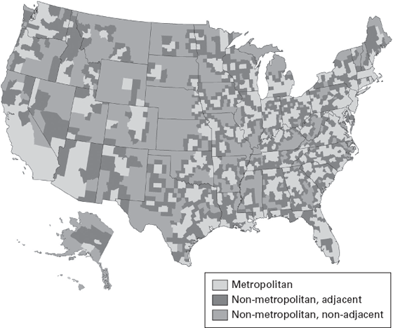
Metropolitan areas include counties with an urban core (city) population of 50,000 or more residents, along with adjacent counties (the suburbs) that link to the urban core by commuting patterns. There are 1,090 metropolitan counties among the 3,141 counties in the United States. All counties that are not within metropolitan areas are grouped together and referred to as nonmetropolitan, even though they differ from one another just as dense urban cores differ from the thinly settled suburbs in metropolitan areas. Our interest is in these 2,051 counties that are not part of metropolitan America (figure 1.1). These are the nonmetropolitan or rural counties that are examined in this chapter. Here the terms “rural” and “nonmetropolitan” are used interchangeably, as are the terms “metropolitan” and “urban.”
Figure 1.1 Metropolitan and adjacent counties.
Source: USDA Economic Research Service, 2004.
Prior research suggests that rural areas near urban areas (adjacent nonmetropolitan counties) have fared better both economically and demographically than counties that are more remote from urban areas (nonadjacent counties). The economic activities in rural counties also differ. Some rural counties depend on farming; others have manufacturing plants; and still others attract tourists to their natural landscapes, lakes, and mountains. Subsets of rural counties are classified using typologies developed by the Economic Research Service of the U.S. Department of Agriculture (USDA, ERS), which group nonmetropolitan counties along economic and policy dimensions (for example, farm counties, manufacturing counties, recreational counties, etc).1
MEASURING RURAL POPULATION CHANGE
Some rural counties have gained population for decades, whereas other counties, including many in the agricultural heartland, have lost people and institutions. A key question is: How does the population of one area grow while another area declines?
Population change in rural areas reflects a balancing act between two demographic forces. The first of these is what demographers call natural increase. Natural increase is the difference between the number of babies born in an area and the number of people who die there (births minus deaths). In the United States as a whole, more babies have been born each year than the number of deaths, so the population has always grown from natural increase. In some parts of rural America, however, there have been times when more people have died than been born. When deaths exceed births, demographers call it natural decrease.
The other force that influences population change is migration. Migration measures the movement of the population from place to place. Migration includes both immigration (when people move between countries) and internal migration within the United States. So, how far do you have to move to be a migrant? If a person moves from one U.S. county to another, he or she is referred to as an internal (or domestic) migrant. If the person stays in the same county, he or she is a mover, but not a migrant.
Demographers are particularly interested in net migration. Net migration is the difference between the number of migrants moving into a county and the number of people who move out. If the number of people migrating in and out of the county is equal, there is no net migration. If one migration stream is larger than the other, then net migration will either increase or decrease the population. Young adults are more likely to migrate than any other age group. When these young adults move to an area, they bring not just themselves but the potential for future population increase through the babies many of them eventually have.
Both natural increase and net migration play important roles in rural population change, but the influence of each varies across time and space. Let’s turn now to the study of the demographic changes that have reshaped rural America through their implications for rural poverty and family well-being.
HISTORICAL POPULATION TRENDS
Throughout most of American history, rural areas grew because migrants moved in and births far exceeded deaths. As the twentieth century progressed, however, these trends changed. The natural increase that sustained rural population growth earlier dwindled as rural women had fewer children. Migration patterns also changed. As the economic and social opportunities in cities grew, rural areas experienced widespread out-migration (figure 1.2). The magnitude of the migration loss varied from decade to decade, but the pattern was consistent: more people left rural areas than arrived. Migration losses from some rural counties were substantial. For example, many farm counties on the Great Plains lost more than half their population from out-migration over the course of several decades. These trends changed in the 1970s when rural population gains exceeded those in metropolitan areas for the first time in the twentieth century, but this rural turnaround was short-lived, ending in the 1980s as widespread out-migration and population decline reemerged. Rural population growth rates rebounded once more in the early 1990s before slowing near the end of the decade (Johnson 2006, 2014). At the dawn of the twenty-first century, population trends in rural America remained unclear.
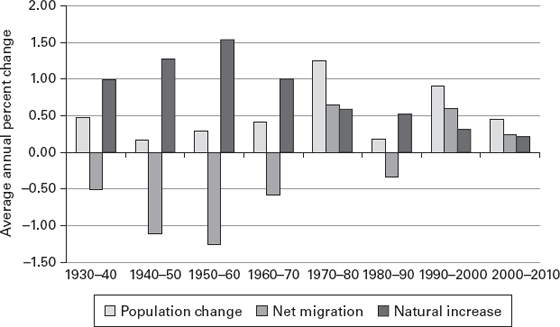
Figure 1.2 Nonmetropolitan demographic change, 1930 to 2010.
Source: U.S. Census 1930–2010 and population estimates.
SOME RURAL AREAS GROW AND OTHERS CONTINUE TO DECLINE IN THE TWENTY-FIRST CENTURY
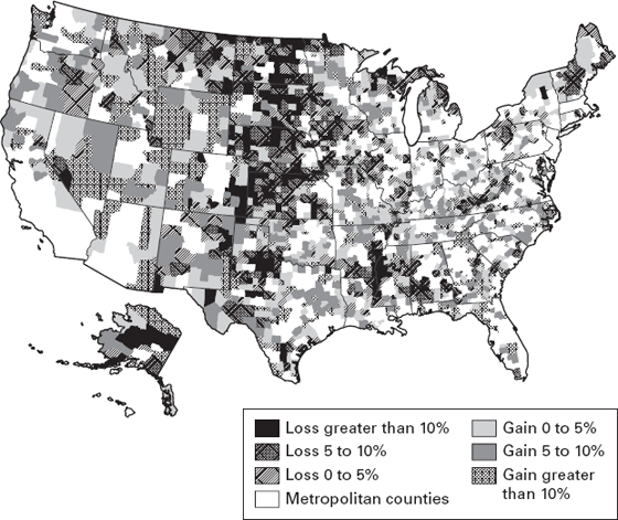
In the first decade of the twenty-first century, patterns of population growth and decline varied widely across rural America (figure 1.3). Population gains were greatest in the West and Southeast, and at the periphery of large urban areas in the Midwest and Northeast. Scattered areas of population gain were evident in recreational regions of the upper Great Lakes, the Ozarks, and northern New England. In contrast, population losses were common in the Great Plains and Corn Belt, in the Mississippi Delta, in parts of the northern Appalachians, and in the industrial and mining belts of New York and Pennsylvania.
Figure 1.3 Nonmetropolitan population change, 2000 to 2010.
Source: U.S. Census Bureau, Census 2000 and 2010.
The slowdown in rural growth has been precipitous. Nonmetropolitan areas gained less than half as many people in the 2000s as they had in the 1990s. Between 2000 and 2010, rural counties gained 2.2 million residents (4.5 percent), to reach a population of 51 million in April 2010. During the 1990s, the rural population gain was nearly twice as large at 4.1 million.
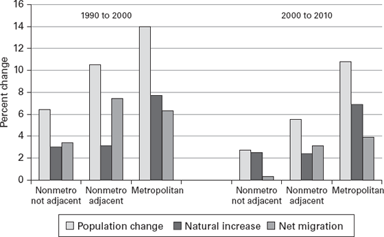
Between 2000 and 2010, population gains were greater in rural counties adjacent to metropolitan areas, just as they were during the 1990s (figure 1.4). Adjacent counties had the advantage of proximity to urban labor markets, as suburban populations on the outer edge of metropolitan areas often spilled over into them. These adjacent counties saw a 5.5 percent population gain between 2000 and 2010. This gain was smaller, however, than it had been during the 1990s. Among more remote nonadjacent counties, the population gain was smaller (2.7 percent), and it was also smaller than during the 1990s.
Figure 1.4 Demographic change in metropolitan and nonmetropolitan areas, 1990–2000 and 2000–2010.
Source: U.S. Census Bureau, Census 1990, 2000, 2010 and the Federal-State Cooperative for Population Estimates (FSCPE).
Population gains in metropolitan areas exceeded those in rural areas during each period. Metropolitan areas grew by 14 percent in the 1990s and by 10.8 percent between 2000 and 2010. A key question is: Why did rural population gains diminish so much after 2000?
The primary cause of the sharply curtailed rural population growth was a slowdown in migration after 2000. During the 1990s, migration accounted for nearly two-thirds of all rural population gain. After 2000, it accounted for less than one-half of the gain. Nonmetropolitan counties gained 2.7 million residents from migration during the 1990s, but only about 1 million between 2000 and 2010. Fewer rural counties experienced migration gains. Only 46 percent of the rural counties gained migrants between 2000 and 2010 compared with 65 percent between 1990 and 2000. Because natural increase in rural areas remained relatively stable over the two decades, this significant reduction in net migration dramatically slowed the rate of population increase. The slowdown was greatest in rural counties that were not adjacent to metro areas. Here the net migration gains were so small that they sharply reduced population growth. Migration gains in more remote areas totaled only 46,000 (0.3 percent), and just 35 percent of these counties gained migrants (Johnson and Cromartie 2006; Johnson 2014). By contrast, in adjacent rural counties, the migration gain was far more sizable at 3 percent (980,000). Overall, 53 percent of the adjacent counties gained migrants between 2000 and 2010.2
With little growth from net migration, natural increase became the major source of nonmetropolitan population growth between 2000 and 2010, accounting for just over half of the gain of 2.2 million rural residents. In remote rural counties, natural increase represented 90 percent of the population gain. In adjacent nonmetropolitan counties, the contributions of natural increase and net migration were more balanced—natural increase accounted for 44 percent of the population increase of 1.7 million.
DIFFERENT TYPES OF COUNTIES HAD DIFFERENT PATTERNS OF DEMOGRAPHIC CHANGE
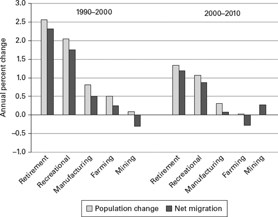
Given the many different kinds of rural counties, it is not surprising that demographic change varied among them. Compare shifts in a county’s dominant industry. Farming and mining no longer monopolize the overall rural economy, but they are still important (see Farming Counties Snapshot). Farming still dominates the local economy of 403 rural counties. These counties are largely at a demographic standstill. Between 2000 and 2010, the population of farming-dependent counties grew by just 0.3 percent (figure 1.5). This minimal population gain was entirely because of a natural increase gain of 3 percent, which was large enough to offset migration loss. In contrast, in the 1990s, farm counties grew by 5 percent, from both natural increase and migration.
Figure 1.5 Demographic change by nonmetropolitan county type, 1990–2010.
Source: U.S. Census 1990–2010 and USDA Economic Research Service, 2004.
Farming Counties: Continuing Population Loss
Rural America was originally settled by people whose livelihood depended on their ability to wrestle food and minerals from the land. The USDA defines 403 farm-dependent counties that represent this traditional rural sector. Among them are Jewell, Osborne, Republic, and Smith counties in Kansas. Situated along the Nebraska-Kansas border and straddling the boundary between the corn and wheat belts, these counties are far removed from the urban scene and have a very large proportion of their labor force engaged in agriculture.
In 1900, nearly 66,000 people lived and farmed in these four counties. The population has declined ever since. By 1990, only 20,700 people remained. The population dropped another 24 percent in the next twenty years, leaving just 15,800 people in 2010. By 2014, the population had diminished further to just 15,400 in the four counties. Young adults have historically left these farm counties in large numbers. In contrast, the older population stays. As a result, all four counties have had more people die than be born in them throughout the last four decades.
These farming-dependent counties do enjoy significant advantages. Unemployment and poverty levels are relatively low. Incomes and housing prices are moderate, producing an affordable standard of living. Residents find these farm counties appealing because they believe their neighbors will help out when needed, people get along, and residents work well together (Hamilton et al. 2008). The continuing loss of people and jobs despite strong social and community capital reflects the dilemma facing many rural farm counties. Without new economic opportunities, the potential for rising poverty levels grows, and three of the four counties have seen poverty levels rise for children in the most recent data.
Mining (which includes oil and gas extraction) is a major force in another 113 counties. Mining counties did better in the 2000s than they had during the 1990s when they suffered significant migration loss. Rising oil prices and new technologies that made the extraction of shale oil financially viable contributed to an influx of energy employees to some mining areas. This resulted in a smaller migration loss and allowed for natural increase to produce a modest population gain of 2.7 percent.
Counties dominated by manufacturing have traditionally been one of the bright spots of rural demographic change (see Manufacturing Counties Snapshot). For decades, efforts by states and the federal government to foster economic growth and development in rural areas focused on expanding the manufacturing base (Johnson 2006).3 The expectation was that a growing manufacturing sector would create jobs that would encourage current residents to stay and attract others to move closer. This strategy worked in the late twentieth century. The 584 rural manufacturing-dominant counties had population gains of 8.1 percent during the 1990s, mostly as a result of migration. However, growth slowed dramatically in the new century. The net population gain was only 3.1 percent between 2000 and 2010. Natural increase accounted for 75 percent of this population gain in manufacturing counties. Migration contributed only modestly to the population growth, considerably less than it had during the 1990s. The globalization of manufacturing coupled with the Great Recession (2007–2010) adversely affected the rural manufacturing sector as the low-skill, low-wage jobs common in some manufacturing facilities shifted offshore or disappeared altogether as technology replaced labor on the shop floor (Johnson 2006, 2014).
Manufacturing Counties: Economic Change and Growing Diversity
Nestled against the Virginia border in the scenic foothills of the Smokey Mountains is Surry County in North Carolina. Surry County has a long history as a rural manufacturing county, mostly in furniture-making and textiles. However, both of these sectors are fading and jobs are disappearing (Johnson 2006, 2014). Poultry processing is growing in the county, as it is in much of the rural Southeast, but jobs are still scarce. Tourism is also on the rise because of the county’s beauty and its proximity to the growing urban areas to the south.
The county has had its demographic ups and downs. Surry’s population grew by 16 percent during the rural turnaround of the 1970s and by 15 percent during the rebound of the 1990s, fueled almost entirely by migration. Growth has slowed down since 2000 as net migration has sharply declined.
Surry County’s recent demographic change illustrates the growing diversity of rural America as well. Hispanics accounted for virtually all of the recent population gain, growing by more than 50 percent between 2000 and 2010 and now representing 10 percent of the population. Poverty is relatively high in the county as well, with nearly 25 percent of children living in families with incomes below the poverty line (Johnson 2006, 2014).
The demographic story is different in rural counties with natural amenities, recreational opportunities, or quality-of-life advantages (see Recreational Counties Snapshot). Counties rich in amenities have consistently been among the fastest growing in rural America. Major concentrations of these counties exist in the mountain and coastal regions of the West, in the upper Great Lakes, in coastal and scenic areas of New England and upstate New York, in the foothills of the Appalachians and Ozarks, and in coastal regions from Virginia to Florida (Johnson and Beale 2002; McGranahan 1999; Economic Research Service [ERS] 2015). These 299 nonmetropolitan recreational counties grew by 10.7 percent between 2000 and 2010.
Recreational Counties: Growth Continuing, but Slowed by Recession
Michigan’s Grand Traverse County exemplifies the fast-growing recreational and retirement destinations discussed in the text. Situated on a beautiful Lake Michigan bay, the county is well known for its crystal clear lakes, ski slopes, golf courses, restaurants, and lodging. It has a well-earned reputation as a year-round recreational center, but its economy is quite diverse.
Grand Traverse amenities attract retirees and the creative classes* seeking an alternative to the hectic pace of urban life. The result has been rapid population increase, from 39,175 in 1970 to 64,273 in 1990, a 64 percent gain in just twenty years. Growth continued in the 1990s with a population gain of 21 percent. Most of the growth came from migration, with a substantial flow from the metropolitan areas of southern Michigan and Chicago. Growth slowed after 2000 as a result of slowing migration, as it has in many recreational areas, especially as the recession deepened. Nonetheless, Grand Traverse County reached a population of 90,800 in 2014.
Grand Traverse’s history of growth has expanded employment opportunities, making it easier for residents to stay and for workers from surrounding areas to move in. The economic opportunities in Grand Traverse County also contribute to low levels of poverty in the area.
This is a smaller gain than during the 1990s, but still substantial compared to farming, mining, and manufacturing counties. There is considerable overlap between these recreational counties and those that attract older adults because of the natural and built amenities that attract vacationers, owners of second homes, and retirees. These retirement counties, like their recreational counterparts, grew rapidly during the 2000s, and the vast majority of that growth came from migration. Some migrants are attracted to the natural and built amenities because they improve their quality of life; other migrants are attracted by economic opportunities generated by these amenity migrants and tourists. The new homes, medical facilities, restaurants, and services they need create many jobs and businesses (see Recreation, Resource Extraction, and Manufacturing Snapshot).
Recreation, Resource Extraction, and Manufacturing: Straddling an Economic Transformation
New Hampshire’s northernmost county, Coos County, has a declining manufacturing and resource extraction base and a growing recreational activity base, producing an unusual demographic profile. For more than a hundred years, wood and paper products were a mainstay of the economy, with large mills employing generations of residents processing the timber of the vast northern forests. Now, nearly all of the mills are gone. Poverty levels have increased recently after decades of relatively low poverty, perhaps reflecting the economic displacements related to the loss of high-paying jobs in the mills.
Situated in a scenic region with ski areas and grand old resorts, Coos County has welcomed generations of vacationers and new amenity migrants. The county is seeking to capitalize on its growing recreational appeal through a countywide advertising effort (Dillon 2011). A great deal is riding on the success of this effort as the county attempts to adapt to the economic and demographic transformation facing rural America in the new century.
Coos County’s demographic history reflects the declines in its manufacturing sector. Currently, the county has 31,700 residents, roughly 2,600 fewer than it had in 1970, and it has lost population in each of the last three decades. There were 3,000 births in Coos County between 2000 and 2010, but more than 4,100 deaths. This produced a natural population loss of 3.3 percent. Between 2000 and 2010, Coos County did gain migrants, partially because of its recreational appeal, but also because two new prisons opened in the county. It has lost migrants again recently.
MIGRATION AND AGING IN PLACE ARE MAKING THE RURAL POPULATION OLDER
Just as migration varies by place, it also varies by age. For decades, migration has drained young adults from rural areas, whereas the older population has both aged in place and grown through retirement-age migration. The combined effect of these migration trends is a reduction in the number of rural young adults and an accelerating aging of the rural population. Fewer young adults means a diminished supply of young workers and fewer children in the next generation. It also means a higher dependency ratio—the ratio of those not in the labor force (children and elderly) to those in the labor force—which puts greater pressure on workers. A growing older population puts greater demands on rural health care facilities and also increases the need for services such as senior centers and assisted living, which are more expensive and difficult to deliver in rural areas where distances are greater and populations are less dense (Chan, Hart, and Goodman 2006).
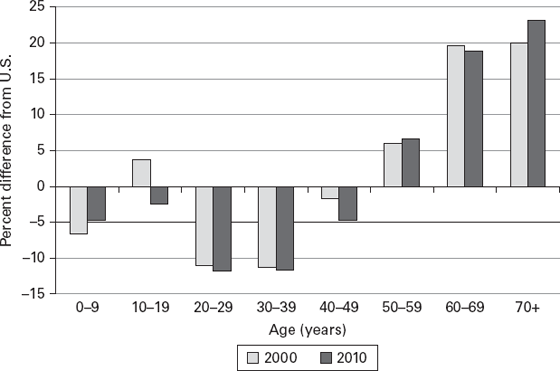
The rural population is already considerably older than that of the United States as a whole, and this trend will likely accelerate in the next several decades. Rural areas have proportionally fewer young adults and fewer children than the overall U.S. population. For example, there were 12 percent fewer people in their twenties and thirties in rural America in 2000 and 2010 than in the United States as a whole (figure 1.6). In contrast, during the same years, the rural population had 20 percent more older adults than the United States as a whole.
Figure 1.6 Age structure differences between nonmetropolitan counties and United States overall, 2000 and 2010.
Source: U.S. Census Bureau, Census 2000 and 2010.
Rural America is older than urban America, primarily because of aging in place among those who already reside there. Rural America has a disproportionately large share of baby boomers born between 1946 and 1964, aged fifty-three to seventy-one in 2017. This group is considerably larger than the cohorts born before or after them—especially in rural America. Having a large population in late middle age has distinct advantages for rural areas right now. It means the working-age population is large compared to those either too old or too young to work. As we look to the future, however, the rural age structure presents significant challenges. As the large baby boomer cohorts continue to age over the next two decades, the number and proportion of seniors in rural America will grow.
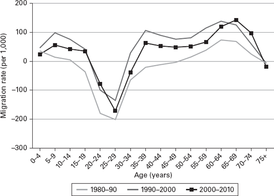
Migration also contributes to the aging of the rural population in two distinctly different ways. Both have implications for the rural future and rural poverty. Rural areas have lost young adults through net out-migration in each of the last three decades (figure 1.7). This long-term loss of young migrants has been substantial. Between 2000 and 2010, rural counties lost 17.1 percent of the residents who would have been age twenty-five to twenty-nine by 2010. Rural areas sustained similar migration losses in the 1980s and 1990s and lost even greater proportions of their young adult population in the 1950s and 1960s.
Figure 1.7 Age-specific net migration rate, nonmetropolitan, 1980–2010.
Source: Winkler et al., 2013.
The economic and social opportunities of urban areas attract rural young people. Some return later in life, but most do not. In some farm counties on the Great Plains, more than half of each generation of young adults has left over the past sixty years. The loss of so many capable young people is a serious concern in many rural areas.
Rural areas tend to gain modest numbers of older adults from migration. Migration gains were evident among those over the age of fifty, with the gains accelerating in the 1990s and 2000s. The scenic amenities, moderate weather, and leisure opportunities available in many of the recreational and retirement counties considered earlier attract older adults. Thus, although most rural counties continue to lose part of their young adult population to out-migration, the older population stays put and in some amenity counties is supplemented by an influx of older migrants. Poverty rates of older adults are significantly lower than those of children and working-age adults, so the changing age distribution in rural America has potential implications for future poverty trends.
THE GROWING DIVERSITY OF RURAL AMERICA
In 2010, 21 percent of the rural population was Hispanic or of a racial group other than white. Although these minorities represent a relatively modest share of the rural population, they accounted for nearly 83 percent of the entire rural population gain between 2000 and 2010. The rural minority population grew by 1.8 million during this decade compared with a gain of just 382,000 (less than 1 percent) among the much more numerous non-Hispanic white population. Rural America remains less diverse than urban America, but minority growth now accounts for most rural population increases, just as it does in urban areas.
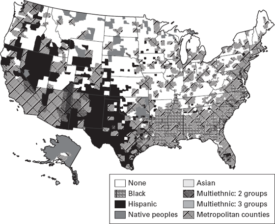
Rural racial diversity is uneven (figure 1.8). Many counties remain overwhelmingly non-Hispanic white. In other rural areas, racial diversity is substantial and increasing rapidly. Large concentrations of African Americans remain in the rural Southeast, bolstered now by a recent influx of black migrants from other regions. Hispanics are spreading out beyond their historic roots in the Southwest into the Southeast and Midwest (Johnson and Lichter 2008). About one-half of the nonmetropolitan Hispanic population now resides outside the rural Southwest (Johnson and Lichter 2008). These resettlement patterns together with Hispanic natural increase have bolstered the diversity of rural America.
Figure 1.8 Nonmetropolitan minority population distribution, 2010.
Source: U.S. Census Bureau, Census 2010.
Hispanics have had a substantial effect on recent rural demographic change. During the 1990s, Hispanics accounted for 25 percent of the entire rural population gain, even though they represented just 3.5 percent of the rural population. This contribution to rural growth accelerated after 2000, when Hispanics accounted for 54 percent of the rural gain although representing only 5.4 percent of the population in 2000. By 2010, the Hispanic population in rural America stood at 3.8 million, or 7.6 percent of the rural population, a gain of 45 percent from 2000. Hispanic migration is now catalyzing large secondary demographic effects on fertility and natural increase (Johnson and Lichter 2008, 2010; Johnson et al. 2014). Most of the rural Hispanic population gain in the 2000s was from natural increase rather than migration (Johnson and Lichter 2008).
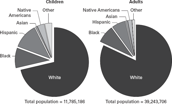
Children are in the vanguard of this growing diversity in nonmetropolitan areas. In rural America, minority children represented 29 percent of the population under age 18 in 2010. In contrast, only 18 percent of the rural adult population belonged to a racial or ethnic minority (figure 1.9). At more than 12 percent in 2010, Hispanics represent the largest share of this minority youth population in rural areas (Johnson and Lichter 2010). These rural patterns are consistent with national trends, although the rural population remains less diverse than the urban population.
Figure 1.9 Nonmetropolitan population by race and Hispanic origin, 2010.
Source: U.S. Census Bureau, Census 2010.
The rural population is also becoming more diverse because the number of white children is declining. There were 940,000 (10 percent) fewer non-Hispanic white children in rural areas in 2010 than there had been in 2000. The number of African American children also declined. In all, there were 515,000 fewer children in rural America in 2010 than there were in 2000. A Hispanic child population gain of 434,000 children (45.1 percent) cushioned the overall loss. The significant loss of white children coupled with a growing Hispanic child population accelerated the diversification of the rural child population.
In 2010, 356 rural counties had more minority children than non-Hispanic white children, and another 178 counties had nearly as many minority children as white children. The concentrations of these rural majority-minority counties are in the Mississippi Delta, the Rio Grande region, the Southeast, and in the northern Great Plains. As the population of minority people grows, children will be the vanguard of this change. Because minority children have higher poverty levels than non-Hispanic white children, there are significant implications for rural poverty. If minority children continue to be at greater risk of poverty as the proportion of all children who are minority grows, child poverty levels are likely to increase significantly.
HOW THE GREAT RECESSION HAS INFLUENCED RURAL DEMOGRAPHIC TRENDS
As we have seen, the population of rural America is always changing. So, what is happening to the rural population right now? The census counts every person in the country but is completed only once every ten years. Census Bureau population estimates are not as accurate as the census, but they still provide a very good idea of how the rural population has changed recently. Data from both of these sources are reflected in the following discussion.
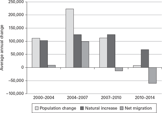
The recent Great Recession was the largest shock to the American economic system since the Great Depression of the 1930s. Because demographic trends are sensitive to economic change, it is important to look briefly at what happened to rural demographic trends during and after the recession. The period from 2000 to 2014 is divided into four segments: the preboom period (April 2000 to July 2004), the economic boom (July 2004 to July 2007), the recession (July 2007 to April 2010), and the postrecession period (April 2010 to July 2014). The National Bureau of Economic Research charted the Great Recession from 2007 to late 2009. The aftermath of the recession, however, is still felt in rural America’s demographic trends.
Rural population growth slowed in the recession and postrecession periods. The annual population gain between 2004 and 2007 was 230,000. The population gain slowed to 112,000 between 2007 and 2010 and to just 8,000 between 2010 and 2014 (figure 1.10). Most of this population slowdown was due to a sharp reduction in net migration during the recession and postrecession years. During the economic boom, rural counties had a net migration gain of 98,000 per year. In contrast, they lost a net 13,000 migrants a year between 2007 and 2010 and had a net migration loss of more than 60,000 a year in the postrecession period. Natural increase also slowed as women had fewer children during the recession and are still having fewer children now. It is unclear whether these births have been delayed because of the lingering effects of the recession on employment, or whether they will be foregone entirely.
Figure 1.10 Demographic change in nonmetropolitan counties, 2000 to 2014.
Source: Census estimate, 2000–2014.
The impact of the recession on migration was spatially uneven (Johnson, Curtis, and Egan-Robertson 2016). Surprisingly, the slowdown was greater in rural counties adjacent to urban areas, where migration gains have historically been the largest due to peripheral growth and spatial sprawl. Paradoxically, in remote rural areas, where historically there has been little if any growth, the effect of the recession on migration was not as great. Remote rural counties suffered migration losses early in the decade, gained migrants during the mid-decade boom, and then, during the recession, the migration gain diminished. The net migration slowdown during the recession was far more modest in these remote rural counties. It is not clear yet whether the slowdown in births and diminished migration to rural America evident in the Great Recession and its aftermath will continue.
SUMMARY AND IMPLICATIONS
The story of demographic change in rural America in the first part of the twenty-first century is one of slowing population growth due to diminished migration and less natural increase. Rural population gains were considerably smaller between 2000 and 2014 than they were during the 1990s. Nonmetropolitan areas grew by barely half as much as they had in the last decade of the twentieth century, and growth slowed even more between 2010 and 2014.
The first decade of the twenty-first century also highlights new patterns of racial and ethnic diversity in rural America. Hispanics, in particular, represent a new source of growth in parts of rural America. The minority population represents just 21 percent of the rural population, but it produced nearly 83 percent of the rural population increase between 2000 and 2010.
Just how demographic changes in rural America affect poverty and family well-being is covered in greater detail throughout the book, but consider just one example of how rural demographic change is pertinent to rural poverty patterns: persistent child poverty. By definition, counties with persistent child poverty have had widespread poverty among their child population for at least the last three decades. Recent research documents the stubborn persistence of such child poverty in large areas of rural America, including the Mississippi Delta and Appalachia (Mattingly, Johnson, and Schaefer 2013). In all, 571 of the 706 U.S. counties with persistent child poverty (81 percent) are in rural America. More than 26 percent of the rural child population resides in counties with persistent child poverty. In comparison, only 12 percent of urban children reside in persistent child poverty counties. The recession has only made it worse, with the proportion of children in poverty rising in these already disadvantaged counties. The demographic changes in rural America over the last decade have done nothing to alleviate persistent poverty, and minority children are at greater risk of poverty than non-Hispanic white children. As we have seen, the minority child population is growing in rural America, and the non-Hispanic white child population is diminishing, increasing rural child poverty. The social and economic isolation fostered by distance and limited transportation in rural America increases the risks many of the rural poor face. Welfare reform, the expansion of government health insurance, and education reforms affect children differently in rural areas than in cities and suburbs (Lichter and Jensen 2002; Lichter and Schafft 2016). A better understanding of how the changing demographic structure of rural America influences the risk of poverty of rural children and adults is needed.
DATA AND METHODS
County population data come from the decennial census for 1990, 2000, and 2010. They are supplemented with data from the Census Bureau’s Population Estimates program, which provides information on births and deaths in each county from 2000 to 2010 (U.S. Census Bureau 2010, 2015). The Census Bureau population, birth, and death estimates for 2010 to 2014 are also used. Estimates of net migration are derived by the residual method, whereby net migration is what is left when natural increase (births minus deaths) is subtracted from total population change.
Data for racial and Hispanic origin of the population are from the 2000 and 2010 censuses. Five ethno-racial groups are identified: (1) Hispanics of any race, (2) non-Hispanic whites, (3) non-Hispanic blacks, (4) non-Hispanic Asians, and (5) all other non-Hispanics, including those who reported two or more races. In some analyses, Native Americans are reported separately. To examine the spatial distribution of different racial and ethnic child populations, the number and percentage of majority-minority counties—those having at least half their child population from minority groups in 2010—and near majority-minority counties—those with between 40 and 50 percent of their children from minority populations—are estimated.
Counties were also classified as having minority concentrations if more than 10 percent of the population was from a specific minority group. Black, Hispanic, Asian, and Native American were the four minority groups that reached the 10 percent threshold in at least one county. Counties that had two or more minority groups reaching the 10 percent threshold were classified as multiethnic.
Data on whether a county is metropolitan or nonmetropolitan come from the Office of Management and Budget, and the classification of rural counties by economic type and recreational and retirement status is from the Economic Research Service of the USDA.
NOTES
1. Five types of rural counties are of particular interest here. Farming counties include those in which a substantial part of the local economy is based on farm earnings and employment. Mining counties are those in which a substantial proportion of local earning and employment comes from mining. Manufacturing counties are those in which a substantial proportion of earnings derives from manufacturing activity. Recreational counties are those in which recreational industries generate considerable earnings and employment and vacation homes are numerous. Retirement counties are those that receive a substantial influx of older migrants. For a fuller description, see USDA Economic Research Service, “Measuring Rurality,” http://www.ers.usda.gov/data-products/rural-urban-continuum-codes.aspx.
2. Immigration contributed more to rural migration gains between 2000 and 2010 than it did during the 1990s. However, even with immigration on the rise, overall migration gains were significantly smaller in rural areas during the first decade of the twenty-first century.
3. Manufacturing is an important component of the rural economy, employing a larger proportion of the rural labor force than it does in urban areas.
REFERENCES
Chan, Leighton, Gary Hart, and David C. Goodman. 2006. “Geographic Access to Health Care for Rural Medicare Beneficiaries.” Journal of Rural Health 22:140–46.
Dillon, Michele. 2011. “Stretching Ties: Social Capital in the Rebranding of Coos County, New Hampshire.” New England Issues Brief. Durham, NH: Carsey Institute.
Hamilton, Lawrence C., Leslie R. Hamilton, Cynthia M. Duncan, and Chris R. Colocousis. 2008. Place Matters: Challenges and Opportunities in Four Rural Americas. A Carsey Institute Report on Rural America. Durham, NH: Carsey Institute.
Johnson, Kenneth M. 2006. “Demographic Trends in Rural and Small Town America.” Reports on Rural America 1(1):1–35. Durham, NH: Carsey Institute.
——. 2014. “Rural Demographic Trends in the New Century.” In Rural America in a Globalizing World, ed. C. Bailey, L. Jensen, and E. Ramson, 311–29. Charleston, SC: University of West Virginia Press.
Johnson, Kenneth M., and Calvin L. Beale. 2002. “Nonmetro Recreation Counties: Their Identification and Rapid Growth.” Rural America 17:12–19.
Johnson, Kenneth M., and John B. Cromartie. 2006. “The Rural Rebound and Its Aftermath: Changing Demographic Dynamics and Regional Contrasts.” In Population Change and Rural Society, ed. W. Kandel and D. L. Brown, 25–49. Dordrecht, Netherlands: Springer.
Johnson, Kenneth M., Katherine J. Curtis, and David Egan-Robertson. 2016. “How the Great Recession Changed U.S. Migration Patterns.” Population Trends in Post-Recession Rural America. Brief 01-16. Madison, WI: Applied Population Laboratory, University of Wisconsin.
Johnson, Kenneth M., and Daniel T. Lichter. 2008. “Natural Increase: A New Source of Population in Emerging Hispanic Destinations in the United States.” Population and Development Review 34:327–46.
——. 2010. “The Growing Diversity of America’s Children and Youth: Spatial and Temporal Dimensions.” Population and Development Review 31(1):151–76.
Johnson, Kenneth M., Andrew P. Schaefer, Daniel T. Lichter, and Luke T. Rogers. 2014. “The Increasing Diversity of America’s Youth: Children Lead the Way to a New Era.” Carsey School of Public Policy National Issue Brief 71. Durham, NH: Carsey School of Public Policy.
Lichter, Daniel T., and Leif Jensen. 2002. “Rural America in Transition: Poverty and Welfare at the Turn of the Twenty-First Century.” In Rural Dimensions of Welfare Reform, ed. B. A. Weber, G. J. Duncan, and L. E. Whitener, 77–110. Kalamazoo, MI: UpJohn Institute.
Lichter, Daniel T., and Kai Schafft. 2016. “People and Places Left Behind: Rural Poverty in the New Century.” In Oxford Handbook of Poverty and Society, ed. D. Brady and L. Burton, 317–40. Oxford: Oxford University Press.
Mattingly, Mary Beth, Kenneth M. Johnson, and Andrew P. Schaefer. 2013. “More Poor Kids in More Poor Places.” Carsey Institute Policy Brief 38. Durham, NH: Carsey Institute.
McGranahan, David. A. 1999. “Natural Amenities Drive Population Change.” Agricultural Economics Report No. 718. Washington, DC: Economic Research Service, U.S. Department of Agriculture.
Winkler, R.L., K. M. Johnson, C. Cheng, P.R. Voss and K.J. Curtis. 2013. County-specific Net Migration by Five-year Age Groups, Hispanic Origin, Race and Sex 2000–2010. CDE Working Paper No. 2013–04. Center for Demography and Ecology, University of Wisconsin—Madison. Madison, WI.