Chapter 14. Performance
Theodore Hong, Imperial College of Science, Technology, and Medicine
We live in the era of speed. Practically as a matter of course, we expect each day to bring faster disks, faster networks, and above all, faster processors. Recently, a research group at the University of Arizona even published a tongue-in-cheek article arguing that large calculations could be done more quickly by slacking off for a few months first, then buying a faster computer:
[B]y fine tuning your slacktitude you can actually accomplish more than either the lazy bum at the beach for two years or the hard working sucker who got started immediately. Indeed with a little bit of algebra we convince ourselves that there exists an optimal slack time s
.[34]
In a world like this, one might well wonder whether performance is worth paying attention to anymore. For peer-to-peer file-sharing systems, the answer is a definite yes, for reasons I will explain in the next section.
Let me first emphasize that by performance, I don’t mean abstract numerical benchmarks such as, “How many milliseconds will it take to render this many millions of polygons?” Rather, I want to know the answers to questions such as, “How long will it take to retrieve this file?” or “How much bandwidth will this query consume?” These answers will have a direct impact on the success and usability of a system.
Fault tolerance is another significant concern. Peer-to-peer operates in an inherently unreliable environment, since it depends on the personal resources of ordinary individual users. These resources may become unexpectedly unavailable at any time, for a variety of reasons ranging from users disconnecting from the network or powering off a machine to users simply deciding not to participate any longer. In addition to these essentially random failures, personal machines tend to be more vulnerable than dedicated servers to directed hacking attacks or even legal action against their operators. Therefore, peer-to-peer systems need to anticipate failures as ordinary, rather than extraordinary, occurrences, and must be designed in a way that promotes redundancy and graceful degradation of performance.
Scaling is a third important consideration. The massive user bases of Napster and of the Web have clearly shown how huge the demand on a successful information-sharing system can potentially be. A designer of a new peer-to-peer system must think optimistically and plan for how it might scale under strains orders of magnitude larger in the future. If local indices of data are kept, will they overflow? If broadcasts are used, will they saturate the network? Scalability will also be influenced by performance: some design inefficiencies may pass unnoticed with ten thousand users, but what happens when the user base hits ten million or more? A recent report from Gnutella analysts Clip2, indicating that Gnutella may already be encountering a scaling barrier, should serve to sound a note of warning.
A note on terminology
We can classify peer-to-peer systems into three main categories, broadly speaking: centrally coordinated, hierarchical, and decentralized.
In a centrally coordinated system, coordination between peers is controlled and mediated by a central server, although peers may later act on information received from the central server to contact one another directly. Napster and SETI@home fall into this category.
A hierarchical peer-to-peer system devolves some or all of the coordination responsibility down from the center to a tree of coordinators. In this arrangement, peers are organized into hierarchies of groups, where communication between peers in the same group is mediated by a local coordinator, but communication between peers in different groups is passed upwards to a higher-level coordinator. Some examples are the Domain Name System (DNS) and the Squid web proxy cache.
Finally, completely decentralized peer-to-peer systems have no notion of global coordination at all. Communication is handled entirely by peers operating at a local level. This usually implies some type of forwarding mechanism in which peers forward messages on behalf of other peers. Freenet and Gnutella are examples in this last category.
In this chapter, when I refer to peer-to-peer systems, I will be talking only about decentralized peer-to-peer. Since the performance issues of centralized systems have been discussed so much, it will be interesting to look at the issues of a fully decentralized system.
Why performance matters
Several factors combine to make decentralized peer-to-peer systems more sensitive to performance issues than other types of software. First, the essential characteristic of such systems is communication—a characteristic that makes them fundamentally dependent on the network. In network communication, as every dial-up user knows, connection speed dominates processor and I/O speed as the bottleneck. Since this situation will most likely persist into the foreseeable future, Moore’s Law (so helpful elsewhere) provides little comfort. The problem is compounded by the highly parallel nature of peer-to-peer: A connection fast enough to talk to one remote peer quickly becomes much less so for ten trying to connect simultaneously. Thus, traffic minimization and load balancing become important considerations.
Second, decentralized systems like Freenet and Gnutella need to use messages that are forwarded over many hops from one peer to the next. Since there is no central server to maintain a master index, it necessarily takes more effort to search through the system to find out where data is. Each hop not only adds to the total bandwidth load but also increases the time needed to perform a query, since it takes a nontrivial amount of time to set up a connection to the next peer or to discover that it is down. As mentioned previously, the latter occurrence can be extremely common in peer-to-peer environments. If a peer is unreachable, TCP/IP can take up to several minutes to time out the connection. Multiply that by several times for retries to other peers and add the time needed to actually send the message over a possibly slow dial-up connection, and the elapsed time per hop can get quite high. It is therefore important to cut down on the number of hops that messages travel.
Third, the balance between resource providers and consumers must be considered. Like their counterparts in the real world, peer-to-peer communities depend on the presence of a sufficient base of communal participation and cooperation in order to function successfully.
However, there will always be those who consume resources without giving any back. Recent analysis by Eytan Adar and Bernardo Huberman at Xerox PARC[35] indicates that as many as 70% of current Gnutella users may be sharing no files at all.
If a high enough proportion of users are free riders, performance degrades for those who do contribute. A substantial decline in performance may impel some contributors to pull out of the system altogether. Their withdrawal worsens the situation further for the remainder, who will have even less incentive to stay, leading to a downward spiral (the well-known "tragedy of the commons”).
To avoid this outcome, system designers must take into account the impact of free riding on performance and devise strategies to encourage higher rates of community participation. Some such strategies are discussed in Chapter 16.
Bandwidth barriers
There has been some progress on the network speed front, of course. Today’s 56-Kbps dial-up lines are a huge improvement on the 300-baud modems of yore. Still, true broadband has been slow to arrive.
Clip2’s analysis of Gnutella is instructive in showing how bandwidth limitations can affect system capabilities. Based on a series of measurements over a period of a month, Clip2 noted an apparent scalability barrier of substantial performance degradation when query rates went above 10 queries per second. To explain this, they proposed the following model. A typical Gnutella query message is about 560 bits long, including TCP/IP headers. Clip2 observed that queries made up approximately a quarter of all message traffic, with another half being pings and the remainder miscellaneous messages. At any given time, Gnutella peers were seen to have an average of three remote peers actively connected simultaneously. Taking these numbers together, we get the following average burden on a user’s link:
       10 queries per second
     ×    560 bits per query
     ×      4 to account for the other three-quarters of message traffic
     ×      3 simultaneous connections
     _______________________________________________________________________
     67,200 bits per second
That’s more than enough to saturate a 56-Kbps link. This calculation suggests that 10 queries per second is the maximum rate the system can handle in the presence of a significant population of dial-up users.
Even when broadband finally becomes widespread, it is unlikely to eliminate the importance of conserving bandwidth and usher in a new era of plenty. Just as building more highways failed to decrease traffic congestion because people drove more, adding more bandwidth just causes people to send larger files. Today’s kilobit audio swapping becomes tomorrow’s megabit video swapping. Hence, bandwidth conservation is likely to remain important for quite some time in the foreseeable future.
It’s a small, small world
In 1967, Harvard professor Stanley Milgram mailed 160 letters to a set of randomly chosen people living in Omaha, Nebraska. He asked them to participate in an unusual social experiment in which they were to try to pass these letters to a given target person, a stockbroker working in Boston, Massachusetts, using only intermediaries known to one another on a first-name basis. That is, each person would pass her letter to a friend whom she thought might bring the letter closest to the target; the friend would then pass it on to another friend, and so on until the letter reached someone who knew the target personally and could give it to him. For example, an engineer in Omaha, on receiving the letter, passed it to a transplanted New Englander living in Bellevue, Nebraska, who passed it to a math teacher in Littleton, Massachusetts, who passed it to a school principal in a Boston suburb, who passed it to a local storekeeper, who gave it to a surprised stockbroker.
In all, 42 letters made it through, via a median number of just 5.5 intermediaries. Such a surprisingly low number, compared to the then-U.S. population of 200 million, demonstrated concretely for the first time what has become popularly known as the small-world effect . This phenomenon is familiar to anyone who has exclaimed “Small world, isn’t it!” upon discovering a mutual acquaintance shared with a stranger.
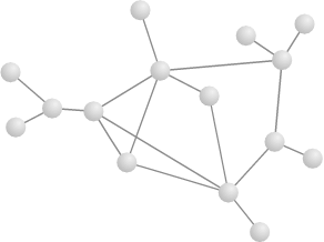
Milgram’s experiment was designed to explore the properties of social networks : the interconnecting bonds of friendship among individuals in a society. One way we can think about social networks is to use the mathematical discipline of graph theory. Formally, a graph is defined as a collection of points (called vertices) that are connected in pairs by lines (called edges).[36] Figure 14.1 shows an example of a graph.
How are graphs related to social networks? We can represent a social network as a graph by creating a vertex for each individual in the group and adding an edge between two vertices whenever the corresponding individuals know one another. Each vertex will have a different number of edges connected to it going to different places, depending on how wide that person’s circle of acquaintances is. The resulting structure is likely to be extremely complex; for example, a graph for the United States would contain over 280 million vertices connected by a finely tangled web of edges.
Computer networks bear a strong resemblance to social networks and can be represented by graphs in a similar way. In fact, you’ve probably seen such a graph already if you’ve ever looked at a connectivity map for a LAN or WAN, although you might not have thought of it that way. In these maps, points representing individual computers or routers are equivalent to graph vertices, and lines representing physical links between machines are edges.
Another electronic analogue to a social network is the World Wide Web. The Web can be viewed as a graph in which web pages are vertices and hyperlinks are edges. Just as friendship links in a social network tend to connect members of the same social circle, hyperlinks frequently connect web pages that share a common theme or topic.
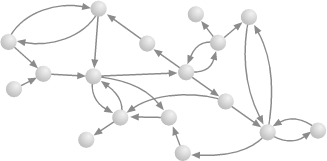
There is a slight complication because (unlike friendships) hyperlinks are one-way; that is, you can follow a hyperlink from a source page to a target page but not the reverse. For Web links, properly speaking, we need to use a directed graph , which is a graph in which edges point from a source vertex to a target vertex, rather than connecting vertices symmetrically. Directed graphs are usually represented by drawing their edges as arrows rather than lines, as shown in Figure 14.2.
Most importantly for our purposes, peer-to-peer networks can be regarded as graphs as well. We can create a Freenet graph, for example, by creating a vertex for each computer running a Freenet node and linking each node by a directed edge to every node referenced in its data store. Similarly, a Gnutella graph would have a vertex for each computer running a Gnutella “servent” and edges linking servents that are connected to each other. These graphs form a useful abstract representation of the underlying networks. By analyzing them mathematically, we ought to be able to gain some insight into the functioning of the corresponding systems.
An excursion into graph theory
There are a number of interesting questions you can ask about graphs. One immediate question to ask is whether or not it is connected. That is, is it always possible to get from any vertex (or individual) to any other via some chain of intermediaries? Or are there some groups which are completely isolated from one another, and never the twain shall meet?
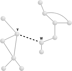
An important property to note in connection with this question is that paths in a graph are transitive . This means that if there is a path from point A to point B, and also a path from point B to point C, then there must be a path from A to C. This fact might seem too obvious to need stating, but it has broader consequences. Suppose there are two separate groups of vertices forming two subgraphs, each connected within itself but disconnected from the other. Then adding just one edge from any vertex V in one group to any vertex W in the other, as in Figure 14.3, will make the graph as a whole connected. This follows from transitivity: by assumption there is a path from every vertex in the first group to V, and a path from W to every vertex in the second group, so adding an edge between V and W will complete a path from every vertex in the first group to every vertex in the second (and vice versa). Conversely, deleting one critical edge may cause a graph to become disconnected, a topic we will return to later in the context of network robustness.
If it is possible to get from any vertex to any other by some path, a natural follow-up question to ask is how long these paths are. One useful measure to consider is the following: for each pair of vertices in the graph, find the length of the shortest path between them; then, take the average over all pairs. This number, which we’ll call the characteristic pathlength of the graph, gives a sense of how far apart points are in the network.
In the networking context, the relevance of these two questions is immediately apparent. For example, performing a traceroute from one machine to another is equivalent to finding a path between two vertices in the corresponding graph. Finding out whether a route exists, and how many hops it takes, are basic questions in network analysis and troubleshooting.
For decentralized peer-to-peer networks, these two questions have a similar significance. The first tells us which peers can communicate with one another (via some message-forwarding route); the second, how much effort is involved in doing so. To see how we can get a handle on these questions, let’s return to the letter-passing experiment in more depth. Then we’ll see if we can apply any insights to the peer-to-peer situation.
The small-world model
The success of Milgram’s volunteers in moving letters between the seemingly disparate worlds of rural heartland and urban metropolis suggests that the social network of the United States is indeed connected. Its characteristic pathlength corresponds to the median number of intermediaries needed to complete a chain, measured to be about six.
Intuitively, it seems that the pathlength of such a large network ought to be much higher. Most people’s social circles are highly cliquish or clustered; that is, most of the people whom you know also know each other. Equivalently, many of the friends of your friends are people whom you know already. So taking additional hops may not increase the number of people within reach by much. It seems that a large number of hops would be necessary to break out of one social circle, travel across the country, and reach another, particularly given the size of the U.S. How then can we explain Milgram’s measurement?
The key to understanding the result lies in the distribution of links within social networks. In any social grouping, some acquaintances will be relatively isolated and contribute few new contacts, whereas others will have more wide-ranging connections and be able to serve as bridges between far-flung social clusters. These bridging vertices play a critical role in bringing the network closer together. In the Milgram experiment, for example, a quarter of all the chains reaching the target person passed through a single person, a local storekeeper. Half the chains were mediated by just three people, who collectively acted as gateways between the target and the wider world.
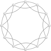
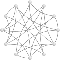
It turns out that the presence of even a small number of bridges can dramatically reduce the lengths of paths in a graph, as shown by a recent paper by Duncan Watts and Steven Strogatz in the journal Nature.[37] They began by considering a simple type of graph called a regular graph , which consists of a ring of n vertices, each of which is connected to its nearest k neighbors. For example, if k is 4, each vertex is connected to its nearest two neighbors on each side (four in total), giving a graph such as the one shown in Figure 14.4.
If we look at large regular graphs in which n is much larger than k, which in turn is much larger than 1, the pathlength can be shown to be approximately n/2k. For example, if n is 4,096 and k is 8, then n/2k is 256—a very large number of hops to take to get where you’re going! (Informally, we can justify the formula n/2k by noticing that it equals half the number of hops it takes to get to the opposite side of the ring. We say only half because we are averaging over all pairs, some of which will be close neighbors and some of which will be on opposite sides.)
Another property of regular graphs is that they are highly clustered, since all of their links are contained within local neighborhoods. To make this notion more precise, we can define a measure of clustering as follows. For the k neighbors of a given vertex, the total number of possible connections among them is k × (k-1)/2. Let’s define the clustering coefficient of a vertex as the proportion (between and 1) of these possible links that are actually present in the graph. For example, in the regular graph of Figure 14.4, each vertex has four neighbors. There are a total of (4 × 3)/2 = 6 possible connections among the four neighbors (not counting the original vertex itself), of which 3 are present in the graph. Therefore the clustering coefficient of each vertex is 3/6 = 0.5.
In social terms, this coefficient can be thought of as counting the number of connections among a person’s friends—a measure of the cliquishness of a group. If we do the math, it can be shown that as the number of vertices in the graph increases, the clustering coefficient approaches a constant value of 0.75 (very cliquish).
More generally, in a non-regular graph, different vertices will have different coefficients. So we define the clustering coefficient of a whole graph as the average of all the clustering coefficients of the individual vertices.
The opposite of the completely ordered regular graph is the random graph . This is just a graph whose vertices are connected to each other at random. Random graphs can be categorized by the number of vertices n and the average number of edges per vertex k. Notice that a random graph and a regular graph having the same values for n and k will be comparable in the sense that both will have the same total number of vertices and edges. For example, the random graph shown in Figure 14.5 has the same number of vertices (12) and edges (24) as the regular graph in Figure 14.4. It turns out that for large random graphs, the pathlength is approximately log n/log k, while the clustering coefficient is approximately k/n. So using our previous example, where n was 4,096 and k was 8, the pathlength would be log 4,096/log 8 = 4—much better than the 256 hops for the regular graph!
On the other hand, the clustering coefficient would be 8/4,096 ≈ 0.002—much less than the regular graph’s 0.75. In fact, as n gets larger, the clustering coefficient becomes practically 0.
If we compare these two extremes, we can see that the regular graph has high clustering and a high pathlength, whereas the random graph has very low clustering and a comparatively low pathlength. (To be more precise, the pathlength of the regular graph grows linearly as n gets larger, but the pathlength of the random graph grows only logarithmically.)
What about intermediate cases? Most real-world networks, whether social networks or peer-to-peer networks, lie somewhere in between—neither completely regular nor completely random. How will they behave in terms of clustering and pathlength?
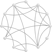
Watts and Strogatz used a clever trick to explore the in-between region. Starting with a 1000-node regular graph with k equal to 10, they “rewired” it by taking each edge in turn and, with probability p, moving it to connect to a different, randomly chosen vertex. When p is 0, the regular graph remains unchanged; when p is 1, a random graph results. The region we are interested in is the region where p is between and 1. Figure 14.6 shows one possible rewiring of Figure 14.4 with p set to 0.5.
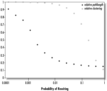
Surprisingly, what they found was that with larger p, clustering remains high but pathlength drops precipitously, as shown in Figure 14.7. Rewiring with p as low as 0.001 (that is, rewiring only about 0.1% of the edges) cuts the pathlength in half while leaving clustering virtually unchanged. At a p value of 0.01, the graph has taken on hybrid characteristics. Locally, its clustering coefficient still looks essentially like that of the regular graph. Globally, however, its pathlength has nearly dropped to the random-graph level. Watts and Strogatz dubbed graphs with this combination of high local clustering and short global pathlengths small-world graphs .
Two important implications can be seen. First, only a small amount of rewiring is needed to promote the small-world transition. Second, the transition is barely noticeable at the local level. Hence it is difficult to tell whether or not your world is a small world, although it won’t take much effort to turn it into one if it isn’t.
These results can explain the small-world characteristics of the U.S. social network. Even if local groups are highly clustered, as long as a small fraction (1% or even fewer) of individuals have long-range connections outside the group, pathlengths will be low. This happens because transitivity causes such individuals to act as shortcuts linking entire communities together. A shortcut doesn’t benefit just a single individual, but also everyone linked to her, and everyone linked to those who are linked to her, and so on. All can take advantage of the shortcut, greatly shortening the characteristic pathlength. On the other hand, changing one local connection to a long-range one has only a small effect on the clustering coefficient.
Let’s now look at how we can apply some of the concepts of the small-world model to peer-to-peer by considering a pair of case studies.
Case study 1: Freenet
The small-world effect is fundamental to Freenet’s operation. As with Milgram’s letters, Freenet queries are forwarded from one peer to the next according to local decisions about which potential recipient might make the most progress towards the target. Unlike Milgram’s letters, however, Freenet messages are not targeted to a specific named peer but toward any peer having a desired file in its data store.
To take a concrete example, suppose I were trying to obtain a copy of Peer-to-Peer. Using Milgram’s method, I could do this by trying to get a letter to Tim O’Reilly asking for a copy of the book. I might begin by passing it to my friend Dan (who lives in Boston), who might pass it to his friend James (who works in computers), who might pass it to his friend Andy (who works for Tim), who could pass it to Tim himself. Using Freenet’s algorithm, I don’t try to contact a particular person. Instead, I might ask my friend Alison (who I know has other O’Reilly books) if she has a copy. If she didn’t, she might similarly ask her friend Helena, and so on. Freenet’s routing is based on evaluating peers’ bookshelves rather than their contacts—any peer owning a copy can reply, not just Tim O’Reilly specifically.
For the Freenet algorithm to work, we need two properties to hold. First, the Freenet graph must be connected, so that it is possible for any request to eventually reach some peer where the data is stored. (This assumes, of course, that the data does exist on Freenet somewhere.) Second, despite the large size of the network, short routes must exist between any two arbitrary peers, making it possible to pass messages between them in a reasonable number of hops. In other words, we want Freenet to be a small world.
The first property is easy. Connectedness can be achieved by growing the network incrementally from some initial core. If each new node starts off by linking itself to one or more introductory nodes already known to be reachable from the core, transitivity will assure a single network rather than several disconnected ones. There is a potential problem, however: If the introductory node fails or drops out, the new node and later nodes connected to it might become stranded.
Freenet’s request and insert mechanisms combat this problem by adding additional redundant links to the network over time. Even if a new node starts with only a single reference to an introductory node, each successful request will cause it to gain more references to other nodes. These references will provide more links into the network, alleviating the dependence on the introductory node. Conversely, performing inserts creates links in the opposite direction, as nodes deeper in the network gain references to the inserting node. Nonetheless, the effect of node failures needs to be examined more closely. We will return to this subject later.
The second property presents more of a challenge. As we saw earlier, it is difficult to tell from local examination alone whether or not the global network is a small world, and Freenet’s anonymity properties deliberately prevent us from measuring the global network directly. For example, it is impossible to even find out how many nodes there are. Nor do we know precisely which files are stored in the network or where, so it is hard to infer much from local request outcomes. We therefore turn to simulation.
Initial experiments
Fortunately, simulation indicates that Freenet networks do evolve small-world characteristics. Following Watts and Strogatz, we can initialize a simulated Freenet network with a regular topology and see how it behaves over time. Suppose we create a network of 1,000 identical nodes having initially empty data stores with a capacity of 50 data items and 200 additional references each. To minimally bootstrap the network’s connectivity, let’s number the nodes and give each node references to 2 nodes immediately before and after it numerically (modulo 1,000). For example, node would be connected to nodes 998, 999, 1, and 2. We have to associate keys with these references, so for convenience we’ll use a hash of the referenced node number as the key. Using a hash has the advantage of yielding a key that is both random and consistent across the network (that is, every node having a reference to node will assign the same key to the reference, namely hash(0)). Figure 14.8 shows some of the resulting data stores. Topologically, this network is equivalent to a directed regular graph in which n is 1,000 and k is 4.
What are the initial characteristics of this network? Well, from the earlier discussion of regular graphs, we know that its pathlength is n/2k, or 1,000/8 = 125. Each node has four neighbors—for example, node 2 is connected to nodes 0, 1, 3, and 4. Of the 12 possible directed edges among these neighbors, 6 are present (from to 1, 1 to 3, and 3 to 4, and from 1 to 0, 3 to 1, and 4 to 3), so the clustering coefficient is 6/12 = 0.5.
A comparable random graph, on the other hand, would have a pathlength of log 1,000/log 4 ≈ 5 and a clustering coefficient of 4/1,000 = 0.004.
Now let’s simulate a simple network usage model. At each time step, pick a node at random and flip a coin to decide whether to perform a request or an insert from that node. If requesting, randomly choose a key to request from those known to be present in the network; if inserting, randomly choose a key to insert from the set of all possible keys. Somewhat arbitrarily, let’s set the hops-to-live to 20 on both insert and request.
Every 100 time steps, measure the state of the network. We can directly calculate its clustering coefficient and characteristic pathlength by examining the data stores of each node to determine which other nodes it is connected to and then performing a breadth-first search on the resulting graph.
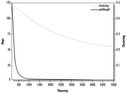
Figure 14.9 shows the results of simulating this model. Ten trials were taken, each lasting 5,000 time steps, and the results were averaged over all trials.
As we can see, the pathlength rapidly decreases by a factor of 20 within the first 500 time steps or so before leveling off. On the other hand, the clustering coefficient decreases only slowly over the entire simulation period. The final pathlength hovers slightly above 2, while the final clustering is about 0.22. If we compare these figures to the values calculated earlier for the corresponding regular graph (125 pathlength and 0.5 clustering) and random graph (5 pathlength and 0.004 clustering), we can see the small-world effect: Freenet’s pathlength approximates the random graph’s pathlength while its clustering coefficient is of the same order of magnitude as the regular graph.
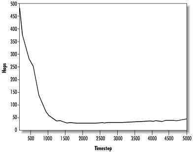
Does the small-world effect translate into real performance, however? To answer this question, let’s look at the request performance of the network over time. Every 100 time steps, we probe the network by simulating 300 requests from randomly chosen nodes in the network. During this probe period, the network is frozen so that no data is cached and no links are altered. The keys requested are chosen randomly from those known to be stored in the network and the hops-to-live is set to 500. By looking at the number of hops actually taken, we can measure the distance that a request needs to travel before finding data. For our purposes, a request that fails will be treated as taking 500 hops. At each snapshot, we’ll plot the median pathlength of all requests (that is, the top 50% fastest requests).
These measurements are plotted in Figure 14.10 and Figure 14.11. Reassuringly, the results indicate that Freenet does actually work. The median pathlength for requests drops from 500 at the outset to about 6 as the network converges to a stable state. That is, half of all requests in the mature network succeed within six hops. A quarter of requests succeed within just three hops or fewer.
Note that the median request pathlength of 6 is somewhat higher than the characteristic pathlength of 2. This occurs because the characteristic pathlength measures the distance along the optimal path between any pair of nodes. Freenet’s local routing cannot always choose the globally optimal route, of course, but it manages to get close most of the time.
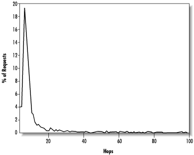
On the other hand, if we look at the complete distribution of final pathlengths, as shown in Figure 14.12, there are some requests that take a disproportionately long time. That is, Freenet has good average performance but poor worst-case performance, because a few bad routing choices can throw a request completely off the track.
Indeed, local routing decisions are extremely important. Although the small-world effect tells us that short routes exist between any pair of vertices in a small-world network, the tricky part is actually finding these short routes.
To illustrate this point, consider a Freenet-like system in which nodes forward query messages to some peer randomly chosen from the data store, rather than the peer associated with the closest key to the query. Performing the same simulation on this system gives the measurements shown in Figure 14.13.
We see that the median request pathlength required now is nearly 50, although analysis of the network shows the characteristic pathlength to still be about 2. This request pathlength is too high to be of much use, as 50 hops would take forever to complete. So although short paths exist in this network, we are unable to make effective use of them.
These observations make sense if we think about our intuitive experience with another small-world domain, the Web. The process of navigating on the Web from some starting point to a desired destination by following hyperlinks is quite similar to the process of forwarding a request in Freenet. A recent paper in Nature by Réka Albert, Hawoong Jeong, and Albert-László Barabási[38] reported that the Web is a small-world network with a characteristic pathlength of 19. That is, from any given web page, it is possible to surf to any other one of the nearly 800 million reachable pages in existence with an average of 19 clicks.
However, such a path can be constructed only by an intelligent agent able to make accurate decisions about which link to follow next. Even humans often fail in this task, getting “lost in the Web.” An unintelligent robot choosing links at random would clearly get nowhere. The only hope for such a robot is to apply brute-force indexing, and the force required is brute indeed: Albert et al. estimated that a robot attempting to locate a web page at a distance of 19 hops would need to index at least a full 10% of the Web, or some 80 million pages.
Simulating growth
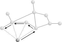
Having taken a preliminary look at the evolution of a fixed Freenet network, let’s now look at what happens in a network that grows over time. When a new node wants to join Freenet, it must first find (through out-of-band means) an initial introductory node that is already in the network. The new node then sends an announcement message to the introductory node, which forwards it into Freenet. Each node contacted adds a reference to the new node to its data store and sends back a reply containing its own address, before forwarding the announcement on to another node chosen randomly from its data store. In turn, the new node adds all of these replies to its data store. The net result is that a set of two-way links are established between the new node and some number of existing nodes, as shown in Figure 14.14.
We can simulate this evolution by the following procedure. Initialize the network with 20 nodes connected in a regular topology as before, so that we can continue to use a hops-to-live of 20 from the outset. Add a new node every 5 time steps until the network reaches a size of 1,000. When adding a new node, choose an introductory node at random and send an announcement message with hops-to-live 10. Meanwhile, inserts and requests continue on every time step as before, and probes every 100 time steps.
It might seem at first that this simulation won’t realistically model the rate of growth of the network, since nodes are simply added linearly every five steps. However, simulation time need not correspond directly to real time. The effect of the model is essentially to interpose five requests between node additions, regardless of the rate of addition. In real time, we can expect that the number of requests per unit time will be proportional to the size of the network. If we assume that the rate at which new nodes join is also proportional to the size of the network, the linear ratio between request rate and joining rate is justified.
Figure 14.15 shows the results of simulating this model. As before, 10 trials were run and the results averaged over all trials.
The results are extremely promising. The request pathlength starts off low, unsurprisingly, since the network is so small initially that even random routing should find the data quickly. However, as the network grows, the request pathlength remains low.
By the end of the simulation, the network is performing even better than the fixed-size simulation having the same number of nodes. Now 50% of all requests succeed within just 5 hops or fewer, while 84% succeed within 20. Meanwhile, the characteristic pathlength and the clustering coefficient are not appreciably different from the fixed case—about 2.2 for the pathlength and about 0.25 for the clustering coefficient.
Simulating fault tolerance
Let’s turn to some aspects of robustness. As mentioned earlier, an important challenge in designing a peer-to-peer system is coping with the unreliability of peers. Since peers tend to be personal machines rather than dedicated servers, they are often turned off or disconnected from the network at random. Another consideration for systems that may host content disapproved of by some group is the possibility of a deliberate attempt to bring the network down through technical or legal attacks.
Taking as a starting point the network grown in the second simulation, we can examine the effects of two node failure scenarios. One scenario is random failure, in which nodes are simply removed at random from the network. The other scenario is targeted attack, in which the most important nodes are targeted for removal. Here we follow the approach of another paper by Albert, Jeong, and Barabási on the fault tolerance of the Internet.[39]
We can model the random failure scenario by progressively removing more and more nodes selected at random from the network and watching how the system’s performance holds up. Figure 14.16 shows the request pathlength plotted against the percentage of nodes failing. The network remains surprisingly usable, with the median request pathlength remaining below 20 even when up to 30% of nodes fail.
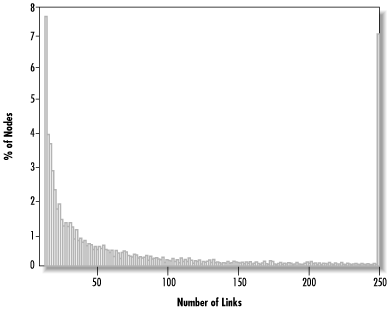
An explanation can be offered by looking at the distribution of links within the network. If we draw a histogram of the proportion of nodes having different numbers of links, as shown in Figure 14.17, we can see that the distribution is highly skewed. Most nodes have only a few outgoing links, but a small number of nodes toward the right side of the graph are very well-connected. (The unusually large column at 250 links is an artifact of the limited data store size of 250—when larger data stores are used, this column spreads out farther to the right.)
When nodes are randomly removed from the network, most of them will probably be nodes with few links, and thus their loss will not hurt the routing in the network much. The highly connected nodes in the right-hand tail will be able to keep the network connected. These nodes correspond to the shortcuts needed to make the small-world effect happen.
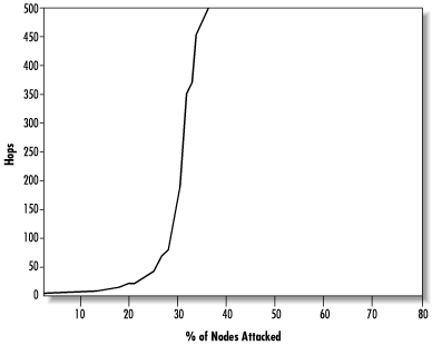
The attack scenario, on the other hand, is more dangerous. In this scenario, the most-connected nodes are preferentially removed first. Figure 14.18 shows the trend in the request pathlength as nodes are attacked. Now the network becomes unusable much more quickly, with the median request pathlength passing 20 at the 18% failure level. This demonstrates just how important those nodes in the tail are. When they are removed, the network starts to fall apart into disconnected fragments.
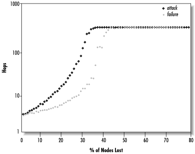
Figure 14.19 shows the contrast between the two failure modes in more detail, using a semi-log scale.
Link distribution in Freenet
Where do the highly connected nodes come from? We can get some hints by trying to fit a function to the observed distribution of links. If we redraw the histogram as a log-log plot, as shown in Figure 14.20, we can see that the distribution of link numbers roughly follows a straight line (except for the anomalous point at 250). Since the equation for a downward-sloping line is:
| y = -kx + b |
where k and b are constants, this means that the proportion of nodes p having a given number of links L satisfies the equation:
| log p = -k log L + b |
By exponentiating both sides, we can express this relationship in a more normal-looking way as:
| p = A × L -k |
This is called a scale-free relationship, since the total number of nodes doesn’t appear in the equation. Therefore it holds regardless of the size of the network, big or small. In fact, scale-free link distributions are another characteristic often used to identify small-world networks.
It turns out that this type of relationship arises naturally from the interaction of two processes: Growth and preferential attachment. Growth just means that new nodes are added over time. Preferential attachment means that new nodes tend to add links to nodes that have a lot of links already. This makes sense because nodes that are well known (i.e., have lots of links) will tend to see more requests and hence will tend to become even better connected.
The impact of free riding
In addition to being robust against node failures, peer-to-peer systems must be able to cope with free riders. Just as in any other social system, there are always those who take from the system without contributing anything back. In the peer-to-peer context, this might mean downloading files but not sharing any for upload, or initiating queries without forwarding or answering queries from others. At best, such behavior just means increased load for everyone else; at worst, it can significantly harm the functioning of the system.
Freenet deals with free riders by simply ignoring them. If a node never provides any files, no other nodes will gain references to it. To the rest of the network, it might as well not exist, so it won’t have any effect on the pathlengths of others’ requests. However, its own requests will contribute to the total bandwidth load on the network while providing no additional capacity. Similarly, if a node refuses to accept incoming connections, other nodes will treat it as though it were down and try elsewhere. Only if a node drops messages without responding will untoward things start to happen, although in that case it is behaving more like a malicious node than a free riding one.
Scalability
Finally, let’s consider Freenet’s scaling properties. In small-world graphs, the characteristic pathlength scales logarithmically with the size of the network, since it follows the random-graph pathlength of log n/log k. That is, a geometric increase in the number of vertices results in only a linear increase in the characteristic pathlength. This means that for example, if k is 3, increasing the size of the network by 10 times would increase the pathlength by just 2. If Freenet’s routing continues to work in large networks, the request pathlength should scale similarly. (Remember that the correlation between the request pathlength and the characteristic pathlength depends on the accuracy of the routing.)
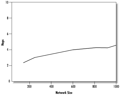
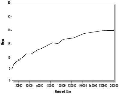
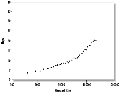
Figure 14.21 shows the results of extending our earlier growth simulation up to 200,000 nodes. As hoped, the request pathlength does appear to scale logarithmically.
We can see the scaling more clearly on the semi-log plot shown in Figure 14.22. On this plot, the data follow approximately straight lines, showing that pathlength is indeed roughly proportional to log(size). The median line has a “knee” where it changes slope at 50,000 nodes. This probably results from data stores becoming filled and could be corrected by creating larger data stores. Note that our data stores were limited to 250 links by the memory requirements of the simulation, whereas real Freenet nodes can easily hold thousands of references. In fact, if we recall the connectivity distribution shown in Figure 14.17, only a small number of high-capacity nodes should be necessary. Even with small data stores, the trend shows that Freenet scales very well: Doubling the network size brings a pathlength increase of only 4 hops.
The number of messages that must be transmitted per request is proportional to the request pathlength, since the latter indicates the number of times a request is forwarded. In turn, the bandwidth used is proportional to the number of messages sent. Thus, the bandwidth requirements of requests should also scale logarithmically in relation to the size of the network. Considering that, in general, the effort required to search for an item in a list grows logarithmically in relation to the size of the list, this is probably the best scaling that can be expected from a decentralized peer-to-peer system.
Case study 2: Gnutella
Gnutella uses a simple broadcast model to conduct queries, which does not invoke the small-world effect. Nonetheless, many of the concepts presented in this chapter can be taken as a useful framework for thinking about Gnutella’s performance, which has been in the trade press so much recently.
In Gnutella, each peer tries to maintain a small minimum number (typically around three) of active simultaneous connections to other peers. These peers are selected from a locally maintained host catcher list containing the addresses of the other peers that this peer knows about. Peers can be discovered through a wide variety of mechanisms, such as watching for PING and PONG messages, noting the addresses of peers initiating queries, receiving incoming connections from previously unknown peers, or using out-of-band channels such as IRC and the Web. However, not all peers so discovered may accept new connections, since they may already have enough connections or be picky about the peers they will talk to. Establishing a good set of connections can in general be a somewhat haphazard process. Further, peers leaving the network will cause additional shuffling as the remaining peers try to replace lost connections.
It therefore seems reasonable to model a Gnutella network by a random graph with a k of 3. Note that such a graph does not necessarily have exactly three edges per vertex. Rather, there will be some distribution in which the probability of finding a vertex having a given number of edges peaks around 3 and decreases exponentially with increasing numbers of edges. We will have more to say about this later.
Gnutella queries propagate through the network as follows. Upon receiving a new query, a peer broadcasts it to every peer that it is currently connected to, each of which in turn will broadcast the query to the peers it is connected to, and so on, in the manner of a chain letter. If a peer has a file that matches the query, it sends an answer back to the originating peer, but still forwards the query anyway. This process continues up to a maximum depth (or “search horizon”) specified by the time-to-live field in the query. Essentially, Gnutella queries perform breadth-first searches on the network graph, in which searches broaden out and progressively cover the vertices closest to the starting point first. (By contrast, Freenet’s style is closer to depth-first search, in which searches are directed deeper into the graph first.)
As before, it is necessary for the network graph to be connected, so that it is possible for any query to eventually reach some peer having the desired data. Achieving complete connectivity is somewhat more difficult than in Freenet because of the random nature of Gnutella connectivity. We can imagine that a random assignment of connections might leave some subset of peers cut off from the rest. However, in practice connectedness appears to hold.
Second, there must again be short routes between arbitrary peers, so that queries will be able to reach their targets before exceeding their depth limits. We turn to simulation to explore these properties.
Initial experiments
Suppose we create a network of 1,000 identical nodes initially sharing no files. To model its connectivity, let’s add 1,500 edges by picking random nodes to be connected, two at a time, and creating edges between them. Topologically, the resulting network will be equivalent to a random graph in which n is 1,000 and k is 3.
Now let’s add data to fill the network, since Gnutella does not have an explicit “insert” or “publish” mechanism. To make this simulation broadly comparable to the Freenet simulation, we’ll randomly generate data items to be stored on 20 nodes each (the equivalent of a Freenet insert with hops-to-live 20). This can be imagined as 20 users independently choosing to share the same file, perhaps a particular MP3. We set the number of different data items added to be the same as the number inserted over the course of the Freenet simulation—that is, about 2,500.
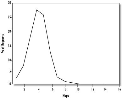
As before, we simulate a simple network usage model. Since a Gnutella network does not evolve organically over time the way a Freenet network does, a single set of probe measurements should suffice. Following our previous method, we perform 300 queries from randomly chosen nodes in the network. The keys requested are chosen randomly from those known to be stored in the network, and the time-to-live is set to infinity, so these queries will always succeed eventually. To gauge the distance a query must travel before finding data, we stop the query as soon as a hit is found and note the number of hops taken to that point. (In the real Gnutella, queries proceed in parallel on a large number of nodes, so it is not practicable to halt them after finding a match on one node.) Figure 14.23 shows the resulting distribution of query pathlengths.
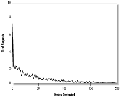
We see that Gnutella queries are satisfied extremely quickly, under both average-case and worst-case conditions. Indeed, the breadth-first search guarantees that the optimal shortest path to the data will always be found, making the query pathlength equal to the characteristic pathlength. However, this is not a true measure of the effort expended by the network as a whole, since queries are broadcast to so many nodes. A better measure is to consider the number of nodes contacted in the course of a query, as shown in Figure 14.24.
A significant number of queries require the participation of 50 nodes, and many even call for 100 or more. It is apparent that the price paid for a quick result is a large expenditure of effort to exhaustively search a significant proportion of the network. Vis-à-vis Freenet, Gnutella makes a trade-off of much greater search effort in return for optimal paths and better worst-case performance.
Fault tolerance and link distribution in Gnutella
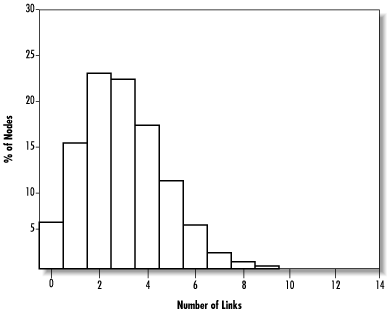
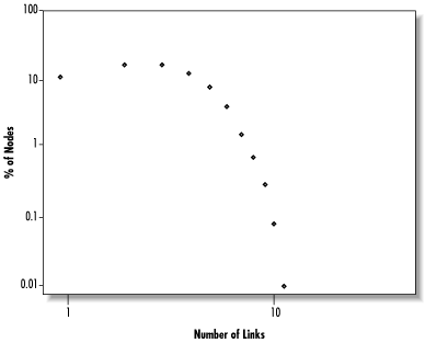
What are Gnutella’s fault-tolerance characteristics? As before, we can consider its behavior under two node failure scenarios: random failure and targeted attack. The distribution of links in Freenet was an important factor in its robustness, so let’s look at Gnutella’s corresponding distribution, shown in Figure 14.25.
Mathematically, this is a “Poisson” distribution peaked around the average connectivity of 3. Its tail drops off exponentially, rather than according to a power law as Freenet’s does. This can be seen more clearly in the log-log plot of Figure 14.26.
Comparing this plot to Figure 14.20, we can see that Figure 14.26 drops off much more sharply at high link numbers. As a result, highly connected nodes are much less of a factor in Gnutella than they are in Freenet.
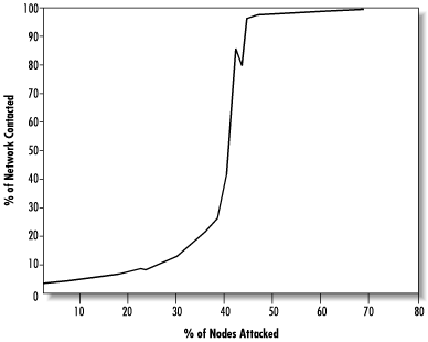
Let’s see how Gnutella behaves under the targeted attack scenario, in which the most-connected nodes are removed first. Figure 14.27 shows the number of nodes contacted per query (as a percentage of the surviving nodes) versus the percentage of nodes attacked. (A request that fails is treated as a value of 100%.) If we compare this plot to Figure 14.18, we can see that Gnutella resists targeted attack better than Freenet does, since the highly connected nodes play less of a role.
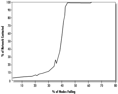
On the other hand, the random failure scenario is the opposite. Figure 14.28 shows the number of nodes contacted versus the percentage of nodes failing. If we compare this to Figure 14.16, Freenet does better.
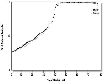
In fact, this occurs because Gnutella performs about the same under both random failure and targeted attack, as can be seen more clearly in Figure 14.29. Here again is a trade-off: Gnutella responds equally to failure and attack, since all of its nodes are roughly equivalent. Freenet’s highly connected nodes enable it to better cope with random failure, but these then become points of vulnerability for targeted attack.
This is brought out in more detail by Figure 14.30, which plots the four scenarios together using an arbitrary scale. We can see that the Freenet failure curve grows much more slowly than the Gnutella curves, while the Freenet attack curve shoots up sooner.
The impact of free riding
Free riding in Gnutella is of more than merely theoretical interest, as indicated by the Xerox PARC paper mentioned earlier. Gnutella is vulnerable to free riders because its peers do not maintain any state information about other peers, so they cannot distinguish free riding from non-free riding peers. In particular, free riding peers will still have queries sent to them even if they never answer any. The presence of free riders will thus “dilute” the network, making queries travel farther before finding data. This can cause queries to fail if the desired data is pushed beyond the search horizon.
Ironically, it may be better for the network if free riding peers drop queries altogether instead of forwarding them, since queries will then simply flow around the free riders (unless portions of the network are completely cut off, of course). This is the opposite of the Freenet situation: Freenet free riders that drop queries are harmful since they kill off those queries, but those that forward queries unanswered actually help the network to route around them later on by propagating information about downstream peers.
Scalability
Finally, let’s consider Gnutella’s scalability. As a random graph, its characteristic pathlength scales logarithmically with the size of the network. Since its breadth-first search finds optimal paths, the request pathlength always equals the characteristic pathlength and also scales logarithmically. We have already seen that these pathlengths are quite low, so the amount of time taken by queries should be manageable up to very large network sizes. This does not accurately reflect their bandwidth usage, however.
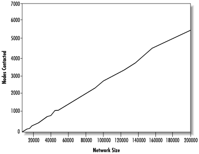
The bandwidth used by a query is proportional to the number of messages sent, which in turn is proportional to the number of nodes that must be contacted before finding data. Actually, this is an underestimate, since many nodes will be sent the same query more than once and queries continue after finding data. Figure 14.31 shows the median number of nodes contacted per query versus network size, up to 200,000 nodes.
We can see that the number of nodes that must be contacted scales essentially linearly, meaning that every doubling of network size will also double the bandwidth needed per query. An alternate way of looking at this is to see that if bandwidth usage is kept lower by limiting search depths, success rates will drop since queries will not be able to reach the data. This may pose a serious scalability problem.
One solution already being explored is to modify Gnutella from a pure decentralized peer-to-peer model to a partly hierarchical model by using super peers . These are special peers that act as aggregators for other peers located “behind” them in the manner of a firewall. Super peers maintain indices of all the files their subordinate peers are sharing, and appear to the rest of the network as though they were sharing those files themselves. When queried for a file, a super peer can route the query directly to the relevant peer without a broadcast. In addition, if one of its subordinates requests a file held by another subordinate, it can satisfy the request immediately without involving the wider network. Super peers thus reduce the effective size of the network by replacing a group of ordinary peers with a single super peer.
From there, it is a short step to imagine “super-super peers” that aggregate queries for super peers, “super-super-super peers,” and so on. Taken to the extreme, this could yield a completely hierarchical search tree like DNS. Such an arrangement would place each peer in successively larger aggregate groups, ultimately ending in a root peer managing the entire network. Searches in such a tree would scale logarithmically; however, it implies a considerable loss of the autonomy promised by peer-to-peer.
Conclusions
Performance is likely to remain an important issue in peer-to-peer systems design well into the foreseeable future. Within the peer-to-peer model, a number of trade-offs can be used to tailor different sets of performance outcomes. Freenet, for example, emphasizes high scalability and efficient searches under average conditions while sacrificing worse-case performance. At the other end of the spectrum, Gnutella sacrifices efficiency for faster searches and better worst-case guarantees. Ideas drawn from graph theory and the small-world model can help to quantify these trade-offs and to analyze systems in concrete terms.
Fault tolerance and free riding are additional challenges to deal with, and here again we can see different approaches. Systems like Freenet that develop specialized nodes can improve their robustness under random failure, but more uniform systems like Gnutella can better cope with targeted attacks. Free riding, a different type of failure mode, needs to be addressed in terms of routing around or otherwise neutralizing uncooperative nodes.
Last but not least, scalability is a crucial concern for systems that hope to make the leap from conceptual demonstration to world-wide usage. For systems that do not inherently scale well, a further set of trade-offs can allow better scalability through a move toward a hierarchical peer-to-peer model, though at the expense of local autonomy.
The peer-to-peer model encompasses a diverse set of approaches. By recognizing the wide range of possibilities available, inventing new ideas and new combinations, and using analytical methods to evaluate their behaviors, system designers will be well-equipped to exploit the power of peer-to-peer.
Acknowledgments
I would like to thank Catherine Reive and the Marshall Aid Commemoration Commission for their help and support. Many thanks also to Ian Clarke for creating Freenet, to Need to Know for bringing it to my attention, to David Molnar for prompting a submission to the ICSI Workshop on Design Issues in Anonymity and Unobservability, and to Sammy Klein, Matt Bruce, and others for reviewing early drafts. Jon Kleinberg’s influence in serendipitously publishing an article on navigation in small-world networks the very week I started writing this was invaluable. Thanks to my thesis advisor, Professor Keith Clark, for putting up with my extracurricular activities. Finally, big thanks go to Andy Oram for putting the whole thing together.
[34] C. Gottbrath, J. Bailin, C. Meakin, T. Thompson, and J.J. Charfman (1999), “The Effects of Moore’s Law and Slacking on Large Computations,” arXiv:astro-ph/9912202.
[35] E. Adar and B.A. Huberman (2000), “Free Riding on Gnutella,” First Monday 5(10), http://firstmonday.org/issues/issue5_10/adar/index.html.
[36] By the way, these graphs have nothing to do with the familiar graphs of equations used in algebra.
[37] D.J. Watts and S.H. Strogatz (1998), “Collective Dynamics of `Small-World’ Networks,” Nature 393, p.440.
[38] R. Albert, H. Jeong, and A. Barabási (1999), “Diameter of the World-Wide Web,” Nature 401, p.130.
[39] R. Albert, H. Jeong, and A. Barabási (2000), “Error and Attack Tolerance of Complex Networks,” Nature 406, p.378.

