It is indeed a feeble light that reaches us from the starry sky. But what would human thought have achieved if we could not see the stars?
—Jean Perrin
CONSIDER FOR A MOMENT development from the egg’s perspective—what a job lies ahead of all those cell divisions and movements, and of making tissue layers, segments, and body parts. We have seen that development proceeds in logical steps, but where are the instructions for each step? How is it that wide stripes are made before narrow ones, or some bones positioned before others? Or how is that some bones are long and thin, and others short and fat? How do the tool kit genes know where to act and when, to shape the development of form? Where are the operating instructions for the tool kit?
To answer these questions, I am going to do two dangerous things. First, I am going to call upon cosmology for an analogy. This is risky because I know very little about the study of the universe, but I have learned that there is a handy analogy between the makeup of the universe and the structure of the genome. And second, I am then going to mix this analogy with another. I will justify committing this writing misdemeanor on the grounds that this chapter presents some of the most challenging, yet also the most revealing and conceptually important information in this book. Bear with me.
For most of its history, astronomy has been about what could be seen in the sky, first with the naked eye and then with ever more powerful telescopes. But while much of what can be seen is always becoming better understood—the formation of stars, the structure of galaxies, and the collapse of suns—cosmologists have only recently confronted the prospect that only a small fraction of the matter in the universe is visible (emitting light or radio waves). The behavior of some visible objects such as galaxies is affected by more abundant, invisible “dark matter” and “dark energy.”
The analogy with genetics is that for decades, because of the simplicity of the genetic code, we biologists have been able to see the “stars” of the genome, to see exactly where genes are encoded in DNA. But we too now appreciate that in most animals’ genomes, the genes that we see occupy just a small fraction of DNA. A much larger part of our DNA consists of sequences that are not part of the simple code for any gene and whose function cannot be deciphered simply by reading the sequence. This is the “dark matter” of the genome. Just as dark matter in the universe governs the behavior of visible bodies, the dark matter in our DNA controls where and when genes are used in development.
This chapter is all about the dark matter in DNA and how, by virtue of controlling how tool kit genes are used, it contains the instructions for making and patterning body parts. These instructions are embedded in the dark DNA as genetic switches (my second analogy). You may not have heard about switches before this book. They have not received nearly as much attention, either in the lab or in the press, as they deserve. But this is more a reflection of the challenge biologists have had in finding them and deciphering how they work, not of their importance. Molecular biologists have only relatively recently been able to peer into the dark and reveal the location and properties of switches. The most surprising and crucial feature of genetic switches is their ability to control very fine details of individual tool kit gene action and anatomy. The anatomy of animal bodies is really encoded and built—piece by piece, stripe by stripe, bone by bone—by constellations of switches distributed all over the genome.
Switches are key actors in both dramas here—development and evolution. These switches draw the beautiful patterns of gene expression we saw in the last chapter. It is the switches that encode instructions unique to individual species and that enable different animals to be made using essentially the same tool kit. And switches are hotspots of evolution—they are the real source of Kipling’s delight—the makers of spots, stripes, bumps, and the like. Part genetic computer, part artist, these fantastic devices translate embryo geography into genetic instructions for making three-dimensional form.
In cosmology, biology, as well as other sciences, the existence of particular entities is detected either directly, by observation, or indirectly, by observing the effects on other entities that are more easily visualized or measured. The evidence for dark matter in the universe is all indirect, based upon observation of the velocities and rotation of galaxies and the deduction that there must be a great deal of mass inside galaxies that cannot be seen. Cosmologists and physicists are not yet sure what dark matter is made of.
Our understanding of dark matter in the genome is much better because we know what it is made of (DNA) and we can isolate it and study its properties both directly and indirectly. One of the most powerful ways to study noncoding “dark” DNA is to hook a piece of it up to a gene that encodes a protein that is easily visualized, such as an enzyme that will make a colored reaction product, or a protein that will fluoresce in a beam of light. By inserting these engineered pieces of DNA back into a genome and then visualizing color patterns in a microscope, we can see what instructions, if any, are contained in a given piece of dark matter (a stripe here, a spot there, etc.). Most dark matter contains no instructions and is just space-filling “junk” accumulated over the course of evolution. In humans, only about 2 to 3 percent of our dark matter contains genetic switches that control how genes are used. I will focus all of this chapter on how genetic switches work to control animal development, and much of the rest of the book on how changes in these switches shape evolution.
I introduced the concept of genetic switches in chapter 3 by describing the genetic system for using lactose and an E. coli bacterium. Recall that in bacteria the synthesis of the enzymes for importing and breaking down lactose is controlled by a genetic switch. The switch is made up of a stretch of DNA sequence that lies just upstream of the genes that encodes these enzymes. When lactose is absent, the lac repressor binds to a specific DNA sequence in the switch and shuts off transcription; when lactose is present, the repressor falls off the switch, allowing the gene for breaking down lactose to be turned on.
In animals, genetic switches are a bit more elaborate. Generally, individual switches in animals are longer sequences of DNA, and they are bound by a larger number and greater variety of proteins. Some of these proteins activate transcription, some repress it. It is by “computing” the inputs of multiple proteins that switches transform complex sets of inputs into the simpler outputs we see as three-dimensional on/off patterns of gene expression, such as the stripes and spots in chapter 4. Importantly, one gene may be regulated by many separate switches such that the gene is used many times and in different places—for example, in the development of the heart, eyes, and fingers (figure 5.1).
The existence of switches expands our picture of how genes work.Usually, when biologists talk about a gene, they mean specifically the stretch of DNA that is decoded into a protein, which in turn does work in cells. Switches are not decoded into anything—their function is regulatory in DNA. To carry out all of its normal functions, a gene depends on information coming from all of its switches. So a gene with three switches has four separable parts, one coding part and three regulatory parts (figure 5.1). Mutations in individual switches can cause some spectacular anatomical effects. I will continue with the typical usage of a “gene” as describing the protein-coding function, and I’ll always make it clear when I am talking about switches.
FIG. 5.1 Genetic switches control where genes are used in body tissues. This gene has switches that control its expression in the heart, eyes, and fingers. The presence of multiple switches, active in different developing body parts, is typical of tool kit genes. DRAWING BY LEANNE OLDS
We have seen that tool kit genes are activated in reference to three-dimensional coordinates within the embryo. But how are the spatial coordinates of the embryo conveyed as instructions to genes, to turn them on and off in precise patterns? The genetic switches act like global positioning system (GPS) devices. Just as a GPS locator in a boat, car, or plane gets a positional fix by integrating multiple inputs, switches integrate positional information in the embryo with respect to longitude, latitude, altitude, and depth, and then dictate the places where gene are turned on and off. I will explain and illustrate how switches work with a few examples. These examples should be thought of as just a few frames out of the whole movie of an animal’s development. The entire show involves tens of thousands of switches being thrown in sequence and in parallel. We aren’t going to worry about every frame; the important thing is to understand the logic and specificity built into these switches.
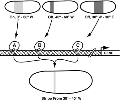
The general function of a switch is to transform existing patterns of gene activity into a new pattern of gene activity. One of the best examples to illustrate the working of a genetic switch is how a band or stripe of longitude is specified along the east-west axis in a fly embryo. Early in development, wide bands of 15-25 cells express specific tool kit proteins at different positions along the axis. Each individual tool kit protein binds to a specific DNA sequence, typically about 6–9 base pairs in length. The recognition of DNA sequences by tool kit proteins is similar to the way a specific key fits into a particular lock. In this case the lock is a particular DNA sequence. I will refer to these as “signature” sequences because they differ for each tool kit protein. Switches that control certain genes contain copies of these signature sequences and are occupied by the respective tool kit proteins in the nuclei of cells, at the longitudes and latitudes in the embryo where the tool kit proteins are present. In the example in figure 5.2, tool kit protein A is expressed from 20° to 60° W, protein B from 40° to 60° W, and protein C from 30° W to 30° E. Protein A is an activator while proteins B and C are repressors of gene X. In general, the rule will be that wherever repressors exist, they will cancel out the activators and the gene will be off. The switch for gene X contains sites for proteins A, B, and C. These sites will be occupied in different combinations along the axis.
FIG. 5.2 Switches integrate multiple inputs to draw a stripe of gene expression. An activator (A) and two repressors (B and C) are expressed at different longitudes; the net output of the switch is a narrow stripe. DRAWING BY JOSH KLAISS
In cells from 90° to 60° W, none of these proteins are on the switch and the gene is off; in cells from 60° to 40° W, both proteins A and B occupy the switch and the gene is off; in cells from 40° to 30° W, only protein A occupies the switch and the gene is on; and in cells from 0° to 30° E, only protein C occupies the switch and the gene is off. By “computing” three longitudinal inputs the switch allows the gene to be on only in a stripe just 10° wide, thus translating three broad patterns of gene expression into one narrow stripe. This stripe is positioned not by a single “on” cue that says “be on from 30° to 40° W,” but by having its boundaries set by a combination of “off” inputs.
You might ask, where do these patterns of tool kit proteins A, B, and C come from? Good question. These patterns are themselves controlled by switches in genes A, B, and C, respectively, that integrate inputs from other tool kit proteins acting a bit earlier in the embryo. And where do those inputs come from? Still earlier-acting inputs. I know this is beginning to sound like the old chicken-and-the-egg riddle. Ultimately, the beginning of spatial information in the embryo often traces back to asymmetrically distributed molecules deposited in the egg during its production in the ovary that initiate the formation of the two main axes of the embryo (so the egg did come before the chicken). I’m not going to trace these steps—the important point to know is that the throwing of every switch is set up by preceding events, and that a switch, by turning on its gene in a new pattern, in turn sets up the next set of patterns and events in development.
Switches may integrate potentially any combination of longitude, latitude, altitude, and depth. An example of a switch that integrates inputs from different axes (figure 5.3) illustrates the actual mechanism of how limb positions are specified in the fly embryo. A switch in the Distal-less limb-building gene integrates both longitude and latitude inputs to place several spots of Dll expression along the main body axis. These inputs are derived from several preexisting patterns of different types of tool kit proteins. One activator is distributed every 15° along the east-west axis within every segment, but only in the southern hemisphere (0°–90° S). Two different repressors are distributed from 30° to 90° S, and at all eastern longitudes, respectively. The integration of these three inputs produces a pattern of Dll expression in small clusters of cells at 90°, 75°, 60°, 45°, 30°, and 15° W, and at 0° to 30° S.
FIG. 5.3 Integration of longitude and latitude determines positions of small clusters of cells that will become limbs. DRAWING BY JOSH KLAISS
The physical integrity of switches is very important to normal development. If a switch is disrupted or broken by mutation, then the proper inputs are not integrated. Many of the spectacular mutants we’ve seen—flies with legs coming out of their head or humans with six fingers or toes—are due to broken switches that turn on tool kit genes in the wrong positions within the embryo or body part.
The makeup of every switch is different. An average-size switch is usually several hundred base pairs of DNA long. Within this span there may be anywhere from a half dozen to twenty or more signature sequences for several different proteins. The response of a switch to a longitude, latitude, altitude, or depth input depends on the presence, number, and local arrangement of signature sequences that are bound by tool kit proteins, which may be deployed along any of these axes or within any specific tissue. The specific patterns drawn by any individual switch are determined by the specific sets of signature sequences encoded in the switch DNA.
In order to appreciate the information residing within a switch and the huge potential variety of switches, I need to provide a bit more detail about the nature of tool kit proteins and these signature sequences in switches. What follows is a brief explanation of the power of using the same tools in different combinations. The exact math isn’t crucial, but understanding the power and efficiency of combinatorial logic is paramount.
The signature sequences recognized by tool kit proteins are short, usually about 6–9 base pairs in length, but can be longer. A lot of different signature sequences can fit into the span of one average-size switch. There are many different possible signature sequences. A 6-base-pair sequence has 4096 permutations of the four DNA bases A, C, G, and T (the math is 46 = 4096), a 7-base-pair-sequence 47 = 16,384 permutations, and an 8-base-pair sequence 48 = 65,536 permutations. A given tool kit protein usually recognizes a family of closely related base sequences. There is some flexibility in the individual bases within a signature sequence but, even with this flexibility, tool kit proteins are highly selective in where they bind along DNA molecules. Different tool kit proteins generally recognize different signature sequences. Here is a very brief list of just a few tool kit proteins that bind to DNA and the signature sequences that they recognize:
Pax-6 (eyeless) |
KKYMCGCWTSANTKMNY |
Tinman |
TCAAGTG |
Ultrabithorax |
TTAATKRCC |
Dorsal |
GGGWWWWCCM |
Snail |
CAGCAAGGTG |
Where:
R = A or G
Y = C or T
K = G or T
M = A or C
S = C or G
W = A or T
N = A, C, G, or T
The whole tool kit of an animal contains several hundred or so different DNA-binding proteins, most with different signature preferences. There are an astronomical number of potential combinations of signature sequences in switches. If we assume a tool kit of 500 DNA-binding proteins in an animal, there are 500 × 500 = 250,000 different pairs of combinations of sequences and tool kit proteins. There are 500 × 500 × 500 = 12,500,000 different three-way combinations and over 6 billion different four-way combinations. These calculations illustrate the power of combinatorial logic of the tool kit and genetic switches. The great variety of switches is a product of using the same signature sequences and tool kit proteins in myriad combinations. One could imagine the alternative would be to have a larger number of tool kit proteins, but it is far more efficient to use 500 proteins in combinations than to encode 250,000 different proteins (which is about ten times more proteins than are encoded in our entire genome).
Allow me one brief aside on the power of combinatorial logic in biology. We have seen this power before in an entirely different context. Our immune systems cope with the enormous diversity of the potential pathogens that live within and around us by making antibody proteins that bind to the proteins, sugars, and fats of these foreign invaders. We have the capacity to make millions of different kinds of antibody proteins. This huge capacity is generated by combining a modest number (a few hundred) of antibody gene regions and antibody chains in different ways, not by encoding millions of different individual antibody genes.
The versatility of switches and of combinatorial logic is very clearly illustrated by experimenting with the DNA sequence content of switches. Simply adding signature sequences to or subtracting them from switches and observing how the patterns they draw change vividly demonstrates the flexibility and power of switches. Mike Levine and his colleagues at the University of California-Berkeley have been leaders in exploring the combinatorial logic of making stripes along both axes in the fly embryo and their work has revealed simple but elegant mechanisms for making patterns.
The basic logic of stripe-making in the early fly embryo was shown in figure 5.2 for a longitudinal stripe. The same general idea of drawing stripes also operates along latitudes. The exact position of a stripe depends upon the strength of the inputs into switches. One way to increase the strength of an input is to add more copies of a signature sequence to a switch. For example, a latitudinal (horizontal) stripe of gene expression that occurs along the southernmost extent of the fly embryo is activated by a tool kit protein whose concentration is graded from south to north. The switch normally contains two signature sequences for this protein. When two copies of a signature sequence for another protein are added to this switch, the stripe expands to more than twice its original width, covering more of the southern hemisphere of the embryo (figure 5.4A).
FIG. 5.4 A. Adding sites for a repressor removes part of the pattern of gene expression. B. Removing sites for a repressor expands the pattern of gene expression. C. Adding sites for a repressor removes part of the pattern of gene expression. DRAWING BY JOSH KLAISS
Alternatively, input can be weakened by reducing the number of signature sequences present in a switch, or it can be eliminated altogether. If these signature sequences are for activators, then the switch can be completely crippled. If the two signature sequences in the switch for the southern stripe above are altered, then this switch is inactivated. However, if signatures for repressor proteins are removed, then the patterns drawn by switches will expand. Section B of figure 5.4 shows another latitudinal stripe pattern drawn by a different switch. This stripe is about 20° wide, extends from 40° to 60° S, and is excluded from the southernmost region of the embryo. The switch controlling this stripe contains four copies of a signature sequence recognized by a repressor that is deployed in the southernmost region of the embryo. If these sites are altered so that the repressors no longer binds to the switch, the pattern drawn by the switch then extends completely to the south pole.
These simple experiments demonstrate how the exact geographic position of a stripe is tuned by the assortment of signature sequence it contains. Getting a switch to draw patterns with respect to both axes is simply a matter of containing signature sequences for tool kit proteins that act along both axes. If one adds a signature sequence for this repressor that is expressed in the southernmost part of the embryo to a longitude stripe element, voilá, the stripe is cut off in the south (figure 5.4C).
All of these simple experiments illustrate how adding, subtracting, or changing just a few bases in a switch can change the patterning output. These nifty demonstrations are important previews of how evolution is shaped by changes in switches by the evolutionary gain or loss of signature sequences. I’ll have much more to say about that later, but it is well worth beginning to think about the possibilities as we delve into the world of genetic switches.
The genes expressed in stripes in the early fly embryo were some of the first to have their switches examined. One of the most surprising discoveries made in taking these genetic switches apart was that individual stripes of multistripe patterns are encoded by separate switches. For example, even though the seven stripes of some tool kit patterns appear very similar and evenly spaced, each stripe is drawn by a different switch that integrates different combinations of longitudinal inputs. This seemed at first like an awful lot of machinery for making just one pattern. But this stripe-by-stripe construction of striped patterns in the fly embryo was the first clue to the general rule that the whole expression pattern of any tool kit gene is actually the sum of many parts, with individual parts controlled by individual switches.
The revelation of how these stripe-making switches work clarified a long-standing question in the study of pattern formation in biological structures. For several decades, mathematicians and computer scientists were drawn to the periodic patterns of body segmentation, zebra stripes, and seashell markings. Heavily influenced by a 1952 paper by the genius Alan Turing (a founder of computer science who helped crack the German Enigma code in World War II), “The Chemical Basis of Morphogenesis,” many theoreticians sought to explain how periodic patterns could be organized across entire large structures. While the math and models are beautiful, none of this theory has been borne out by the discoveries of the last twenty years. The mathematicians never envisioned that modular genetic switches held the key to pattern formation, or that the periodic patterns we see are actually the composite of numerous individual elements.
A gene not only may have multiple switches for different subpatterns of expression at a given time, but will frequently have different switches that control entirely different patterns in different tissues and at different stages in development. Tool kit genes are rarely, if ever, devoted to a single developmental operation. Rather, these tools are used and reused again and again in development in different contexts to shape the growing embryo. Switches endow individual tool kit genes with great versatility. Virtually every tool kit gene is controlled by multiple switches. Ten switches or more is not uncommon, and we don’t know what the upper limit, if any, may be.
The building of bodies and body parts is accomplished by the sum of operations governed by individual switches. The large and complex skeletal anatomy of vertebrates is actually encoded and constructed, bone by bone, by arrays of switches nested around a host of tool kit genes. One family of important tool kit proteins for skeletal development, the Bone Morphogenetic Proteins (BMPs), is so called because they have the property of promoting cartilage and bone formation. The regulation of one member of this family, the BMP5 gene, vividly illustrates how parts of anatomy are encoded in pieces through separate switches.
All around the BMP5 gene, there are switches. There are separate switches for BMP5 expression in ribs, limbs, fingertips, the outer ear, the inner ear, vertebrae, thyroid cartilage, nasal sinuses, the sternum, and more (figure 5.5). The same protein is being produced in all of those different patterns, places, and times—the specificity of each operation and the complexity of the overall pattern are entirely due to the array of switches. The existence of separate switches for each of these parts illustrates the fine-tuning control that is available for the construction and shaping of every body part.
The spectacular diversity and exquisite geographic specificity of switches derive from the use of combinatorial logic. Because the combination of inputs determines the output of a switch, and the potential combinations of inputs increase exponentially with each additional input, the potential outputs of switches are virtually endless. Imagine the possibilities of combining bands, stripes, lines, spots, dots, and patches of activators and repressors and the ability to draw these in any place, in any tissue, and in any combination. All kinds of patterns are possible, and switches that draw an enormous variety of patterns have been found in individual animal genomes. For any coordinate or sets of coordinates, switches can and do draw just about any geometric pattern of gene expression.
FIG. 5.5 Individual switches control the expression of the BMP5 gene in different parts of the developing mouse embryo. ADAPTED FROM DAVID KINGSLEY, HOWARD HUGHES MEDICAL INSTITUTE AND STANFORD UNIVERSITY; DRAWING BY JOSH KLAISS
While it is true that the number of potential combinations of inputs and signature sequences is enormous, the actual set of switches in any animal is finite. And not every switch is entirely different. In order to coordinate development, especially the making of particular cell types that have dedicated functions, switches in different genes often share one or more inputs and signature sequences in common. For example, in order to function as muscle cells, a set of proteins must be produced that enable the cells to contract, to rapidly utilize energy sources, and to efficiently remove waste during muscle activity. The genes encoding these proteins are activated in the muscle cell by switches with common signature sequences recognized by the same tool kit protein. The same is true in other specific cell types—neurons, photoreceptor cells in the eye, pancreatic cells, the pituitary, etc. Organ functions commonly depend upon one or a few tool kit proteins that throw sets of switches belonging to many genes located throughout the genome.
With a good feel now for how genetic switches work, let’s turn to how they fit into the major trends of animal design, and to start thinking about how animals evolve. The fundamental feature of large, complex animals such as arthropods and vertebrates is their modular construction from repeating parts. Understanding how switches are used to make repeating parts into different forms with different functions is central to understanding the making and evolution of our favorite animals.
We saw in the last chapter that the expression of different Hox genes occurs in the different segments and appendages of arthropods, and the different rhombomeres and somites of vertebrates. The pattern and function of each repeated part depend upon the unique Hox gene or combination of Hox genes acting in each segment, appendage, somite, or rhombomere. The establishment of these Hox “zones” and their subsequent action in sculpting the different forms of repeated parts is the fundamental genetic logic upon which the modular forms of large, bilateral animals are built.
This genetic logic relies on genetic switches at two levels. One set of switches belongs to the Hox genes themselves. These switches activate each Hox gene in different zones that will become different modules of the animal. Another set of switches contain signature sequences that are recognized by Hox proteins and that control how other genes are expressed in different modules.
In both arthropods and vertebrates, the Hox genes are deployed in zones along the main body axis. The distinct zones of each Hox gene’s expression domain are governed by genetic switches, and separate switches control Hox gene patterns in different tissues such as the hind-brain, neural tube, somites, and limb buds in vertebrates and the epidermis and nerve cord in arthropods. Because of the logic of these switches, the cells that belong to one module express different Hox proteins or combinations of Hox proteins than those in adjacent modules. The different forms of each module—brain rhombomere or somite, arthropod segment or appendage—are sculpted by Hox proteins acting on other genes.
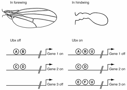
The general logic of how Hox proteins sculpt the different morphologies of repeated parts is most easily illustrated in insects. Along the main body axis, most segments are patterned differently and bear different structures. For example, the first thoracic segment bears no wings, the second thoracic segment bears the large forewings, and the third thoracic segment bears the smaller hindwings used for balance. No Hox protein is expressed in forewing cells but all hindwing cells express Ubx (because a set of switches in the Ubx gene activate it in the third thoracic segment and hindwing). The difference in appearance between the hindwing and forewing is due to Ubx action.
Ubx sculpts the form of the hindwing by acting on the switches of genes that pattern the wings. It turns off genes that promote the formation of forewing features (veins and other structures) and turns on genes that promote hindwing features. The switches in these genes must integrate multiple inputs (and contain signature sequences for each). If we take a snapshot of a handful of switches and gene activity and contrast their states in the forewing and hindwing, the basic logic that we find is that Ubx acts on a subset of switches to shape the hindwing to be different from the forewing (figure 5.6).
The same logic applies to making different rhombomeres, different limb types in arthropods, vertebrae, and ribs. The different final forms of these serially reiterated structures are sculpted by Hox proteins that determine which subsets of limb-, rhombomere-, vertebrae-, or rib-patterning genes are active at each position along the body axis.
FIG. 5.6 Alternative states of gene expression in the forewing and hindwing are controlled by a Hox protein. The solid lines represent switches, the letters different regulatory proteins (U stands for Ubx). The different forms of the two wings result from different sets of genes being active in each. DRAWING BY JOSH KLAISS
I have illustrated the way genetic switches work by focusing on one switch of a given gene, the various switches of one gene, or the assortment of switches controlled by a common protein. But every switch or protein I have described and each pattern I have shown is just a still photo—adding up to relatively few frames in the whole course of an animal’s development. The entire story of making an animal has many, many more frames—it is one hell of a movie with nonstop action.
The forms of animals and their body parts are never the result of the action of a single switch or protein. Body parts, tissues, and cell types are the products of large numbers of switches and proteins that organize patterns in time and space, and of proteins and other molecules that endow cells and tissues with their physiological and mechanical properties. The developmental steps executed by individual switches and proteins are connected to those of other genes and proteins. Larger sets of interconnected switches and proteins form local “circuits” that are part of still larger “networks” that govern the development of complex structures. Animal architecture is a product of genetic regulatory network architecture.
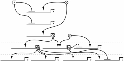
This circuit and network wiring or logic can be illustrated with the same sort of diagrams used for electrical circuits or logic problems. Each switch is a decision point, one node in the genetic circuitry. Figure 5.7 shows a set of interconnected circuits that involve a small number of activators, repressors, switches, and genes. This again is a model of just a few parts of a much bigger picture. My guess is that I would need at least one thousand pages to write out the logic of making a fly, and several thousand pages to write out the making of a human. Regulatory networks in vertebrates are more numerous (we have three times as many cell types as flies or other invertebrates), but not really any more complicated.
FIG. 5.7 A genetic wiring diagram of regulatory logic. Activators (circled letters) and repressors (squared letters) act on switches (solid lines). Arrows indicate activation effects, lines ending with a perpendicular line denote repression. Multiple tiers of activators and repressors are usually involved in building and patterning any structure. DRAWING BY JOSH KLAISS
Biologists are still coming to grips with the profound importance of genetic switches. For several decades, we have been able to read the genetic code and see exactly how and where protein sequences are encoded in DNA. The common view from this protein-centric perspective was that genes were bodies of information in the vast expanse of DNA, with all that space around and between genes being largely empty of information. The belief was also widespread that differences between animals would largely be a matter of changes in the number and sequence of genes. But now we are beginning to understand that there can be many genetic switches surrounding a gene. And genome sequencing has shown us that mice and humans have nearly identical numbers and kinds of genes (about 25,000 each). So, given that the coding sequences are so similar, it is time to explore the surrounding switches to understand their roles in evolution.
The glimpses here into the logic and great potential diversity of genetic switches prepare us to start thinking about their contribution to the evolution of animal diversity. The great paradox raised by the discovery of similar sets of tool kit genes in disparate animals is how the same genes can be used to build such different forms. The discovery of arrays of switches that enable individual tool kit genes to be used again and again in one animal, and to be used in slightly or dramatically different ways in serially repeated structures, is key to solving this paradox.
It is a small leap from understanding how switches control development to anticipating how they have shaped evolution. Switches enable the same tool kit genes to be used differently in different animals. Because individual switches are independent information-processing units, evolutionary changes in one switch of a tool kit gene or in a switch controlled by a tool kit protein can alter the development of one structure or pattern without altering other structures or patterns. This is the key to the evolution of modular bodies and body parts—how we, for example, can evolve an opposable thumb, or flies can evolve a special hindwing. Many of the evolutionary mysteries I will now explore in the second part of the book, from the great burst of diversity in animal forms that marks the Cambrian Explosion to the wonderful variety of butterflies or mammals living today, were shaped by evolutionary changes in genetic switches.