APPENDIX F. SUMMARY OF PROPERTIES AND KEY THEOREMS

    Basic probability

        Definition 2-3a

A probability system (or probability space) consists of the triple

1. A basic space S of elementary outcomes (elements)

2. A class of events (a sigma field of subsets of S)

3. A probability measure P(·) defined for each event A in the class and having the following properties:

(P1) P(S) =1 (probability of the sure event is unity)

(P2) P(A) ≥ 0 (probability of an event is nonnegative)

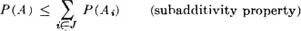
(P3) If = {A_i: i ∈ J} is a countable partition of A (i.e., a mutually exclusive class whose union is A), then

Further properties

(P8) Let = {B_i: i ∈ J} be any countable class of mutually exclusive events. If the occurrence of the event A implies the occurrence of one of the B_i (i.e., if A ⊂ B_i), then .

(P9) If {A_n: 1 ≤ n < ∞} is a decreasing or an increasing sequence of events whose limit is the event A, then .

(P10) Let = {A_i: i ∈ J} be any countable class of events, and let A be the union of the class. Then

Conditional probability

Definition 2-5a

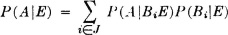
If E is an event with positive probability, the conditional probability of the event A, given E, written P(A|E), is defined by the relation

(CP1) Product rule for conditional probability

(CP2) Let = {B_i: i ∈ J} be any countable class of mutually exclusive events, each with positive probability. If the occurrence of the event A implies the occurrence of one of the B_i (i.e., if ), then

(CP3) Bayes’ rule. Let = {B_i: i ∈ J} be any countable class of mutually exclusive events, each with positive probability. Let A be any event with positive probability such that . Then

(CP4) P(A₁A₂ … A_n|E) = P(A₁|E)P(A₂|A₁E) … P(A_n|A₁ … A_{n − 1}E)

(CP5) Let = {B_i i ∈ J} be any finite or countably infinite class of mutually exclusive events, each with positive probability. If the occurrence of the event A implies the occurrence of one of the B_i (i.e., if 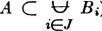), then

Stochastic independence

Definition 2-6a

Two events A and B are said to be (stochastically) independent iffi the following product rule holds:

Definition 2-6b

A class of events = {A_i: i ∈ J}, where J is a finite or an infinite index set, is said to be an independent class iffi the product rule holds for every finite subclass of .

Theorem 2-6E

Suppose = {A_i: i ∈ I} is any class of events. Let {_j: j ∈ J} be a family of finite subclasses of such that no two have any member event A_i in common. Let B_j be the intersection of all the sets in _j. Put = {B_j: j ∈ J}. Then is an independent class iffi every class so formed is an independent class.

Theorem 2-6F

If = {A_i: i ∈ J} is an independent class, so also is the class ′ obtained by replacing the A_i in any subclass of by either , S, or A_i^c. The particular substitution for any given A_i may be made arbitrarily, without reference to the substitution for any other member of the subclass.

Theorem 2-6G

Suppose = {A_i: i ∈ I} and = {B_i: j ∈ J) are countable disjoint classes whose members have the property that any A_i is independent of any B_i; that is, P(A_iB_j) = P(A_i)P(B_i) for any i ∈ I and j ∈ J. Then the events

Theorem, 2-8A

Suppose {A₁, A₂, … A_n, B₁, B₂, …, B_m} is an independent class, and let

be boolean functions of the indicated events. Then F and G are independent events.

Boolean functions of events

Definition 2-7d

A boolean function F = f(A, B, …) of a finite class of sets is a set obtained by a finite number of applications of the operations of union, intersection, and complementation to the members of the class.

Theorem 2-7A Minterm Expansion Theorem

Any boolean function F = f(A_N−1, A_N−2, …, A₁, A₀) may be expressed as the disjoint union of an appropriate subclass of the minterms m_i generated by the class {A_N−1, A_N−2, … A₁, A₀}. In symbols, , where J_F is a suitable index set.

Random variables and events

Theorem 3-1A

Suppose X(·) is a mapping carrying elements of the domain S into elements t in the range T. Then

1. The inverse image of the union (intersection) of a class of the t sets is the union (intersection) of the class of inverse images of the separate t sets.

2. The inverse image of the complement of a t set is the complement of the inverse image of the t set.

3. If a class of t sets is a disjoint class, the class of the inverse images is a disjoint class.

4. The relation of inclusion is preserved by the inverse mapping.

Theorem 3-1B

If the function X(·) is such that {: X() ≤ t} is an event for each real t, then X⁻¹(M) is an event for each Borel set M.

Definition 3-1a

A real-valued function X(·) from the basic space S to the real line R is called a (real-valued) random variable iffi for each real t it is true that {: X() ≤ t} is an event.

Definition 3-2a

The probability measure P_X(·) defined on the class of Borel sets _R by

is called the probability measure induced by the random variable X(·).

Discrete random variables

Definition 3-3a

A random variable X(·) whose range T consists of a finite set of values is called a simple random variable. If the range T consists of a countably infinite set of distinct values, the function is referred to as an elementary random variable. The term discrete random variable is used to indicate the fact that the random variable is either simple or elementary.

Definition 3-3b

The discrete random variable X(·) is said to be in canonical form iffi it is written

where T = {t_i: i ∈ J} is a set of distinct constants and {A_i: i ∈ J} is a partition.

Definition 3-3c

The discrete random variable X(·) is said to be in reduced canonical form iffi it is written

where T′ = {t_i: i ∈ J} is a set of distinct, nonzero constants and {B_i: i ∈ J) is a disjoint class.

Theorem 3-3A

A bounded, nonnegative random variable X(·) can be represented as the limit of a nondecreasing sequence of simple functions. The convergence of this sequence is uniform in over the whole basic space S.

Probability distribution functions

Definition 3-4a

For any real-valued random variable X(·), we define the distribution function F_X(·) by the expression

for each real t.

Definition

The function

is called the unit step function. The function has been left undefined at t = 0. If we define the function to be continuous from the right, we use the symbol u₊(·).

(F1) F_X(t) is monotonically increasing with increasing t.

(F2)

(F3) P(a < X ≤ b) = P(X ∈ (a, b]) = F_X(b) − F_X(a)

(F4) F_X(·) has a jump discontinuity of magnitude δ > 0 at t = a iffi P(X = a) = δ. F_X(·) is continuous at t = a iffi P(X = a) = 0.

(F5) F_X(·) is continuous from the right.

Definition 3-4b

If the probability measure P_X(·) induced by the real-valued random variable X(·) is such that it assigns zero probability to any point set of Lebesgue measure (generalized length) zero, the probability measure and the probability distribution are said to be absolutely continuous (with respect to Lebesgue measure). In this case, the random variable is also said to be absolutely continuous.

Definition 3-4c

If the probability measure P_X(·) induced by the real-valued random variable X(·) is absolutely continuous, the function f_X(·) defined on the real line such that

is called the probability density function for X(·).

Definition 3-5a

The probability measure P_XY(·) defined on the Borel sets in the plane is called the joint probability measure induced by the joint mapping (t, u) = Z() = [X, Y](). The probability mass distribution is called the joint distribution. The probability measures P_XY(· × R₂) = P_X(·) and P_XY(R₁ × ·) = P_Y(·) are called the marginal probability measures induced by X(·) and Y(·), respectively. The corresponding probability mass distributions are called the marginal distributions.

Definition 3-6a

The function F_XY(·, ·) defined by

F_XY(t, u) = P(X ≤ t, Y ≤ u)

is called the joint distribution function for X(·) and Y(·). The special cases F_XY(·, ∞) and F_XY(∞, ·) are called the marginal distribution functions for X(·) and for Y(·), respectively.

Definition 3-6b

If the joint probability measure P_XY(·) induced by X(·) and Y(·) is absolutely continuous, a function f_XY(·, ·) exists such that for each Borel set Q on the plane. The function f_XY(·, ·) is called a joint probability density function for X(·) and Y(·).

Independent random variables

Definition 3-7a

The random variables X(·) and Y(·) are said to be (stochastically) independent iffi, for each choice of Borel sets M and N, the events X⁻¹(M) and Y⁻¹(N) are independent events.

Definition 3-7b

A class {X_i(·): ∈ J} of random variables is said to be an independent class iffi, for each class {M_i: i ∈ J} of Borel sets, arbitrarily chosen, the class of events {X_i⁻¹(M_i): i ∈ J} is an independent class.

Theorem 3-7 A

Random variables X(·) and Y(·) are independent iffi

for each Borel set M in R₁, and N in R₂.

Theorem 3-7B

Any two real-valued random variables X(·) and Y(·) are independent iffi, for all semi-infinite, half-open intervals M_t and N_u, defined by M_t = {: X() ≤ t} and N_u = {: Y() ≤ u},

By definition, the latter condition is equivalent to the condition

for all such half-open intervals,

Theorem 3-7C

Two random variables X(·) and Y(·) are independent iffi their distribution functions satisfy the product rule

If the density functions exist, then independence of the random variables is equivalent to the product rule f_XY(t, u) = f_X(t)f_Y(u) for the density functions.

Theorem 3-7 D

Suppose X(·) and Y(·) are independent random variables, each of which is non-negative. Then there exist nondecreasing sequences of nonnegative simple random variables {X_n(·): 1 ≤ n < ∞ } and {Y_m(·): 1 ≤ m < ∞} such that

and. {X_n(·), Y_m(·)} is an independent pair for any choice of m, n.

Functions of random variables

Definition 3-8a

If g(·) is a real-valued function of a single real variable t, the function Z(·) = g[X(·)} is defined to be the function on the basic space S which has the value v = g(t) when X() = t.

Definition 3-8b

Let g(·) be a real-valued function, mapping points in the real line R₁ into points in the real line R₂. The function g(·) is called a Borel function iffi, for every Borel set M in R₂, the inverse image N = g⁻¹(M) is a Borel set in R₁. An exactly similar definition holds for a Borel function h(·, ·), mapping points in the plane R₁ × R₂ into points on the real line R₃.

Theorem 3-8A

If W(·) is a random vector and g(·) is a Borel function of the appropriate number of variables, then Z(·) = g[W(·)] is a random variable measurable (W).

Theorem 3-8B

If {X_i(·): i ∈ J} is an independent class of random variables and if, for each i ∈ J, W_i(·) is (X_i) measurable, then {W_i(·): i ∈ J} is an independent class of random variables.

Almost-sure relationships

Definition 3-10a

Two events A and B are said to be equal with probability 1, designated in symbols by

We also say A and B are almost surely equal.

Definition 3-10b

Two classes of events and are said to be equal with probability 1 or almost surely equal, designated = [P], iffi their members may be put into a one-to-one correspondence such that A_i = B_i [P] for each corresponding pair.

Definition 3-10d

A property of a random variable or a relationship between two or more random variables is said to hold with probability 1 (indicated by the symbol [P] after the appropriate expression) iffi the elements for which the property or relationship fails to hold belong to a set D having 0 probability. In this case we may also say that the property or the relationship holds almost surely.

A property or relationship is said to hold with probability 1 on (event) E (indicated by “[P] on E”) iffi the points of E for which the property or relationship fails to hold belong to a set having 0 probability. We also use the expression “almost surely on E.”

 

Mathematical expectation

Definition 5-1a

If X(·) is a real-valued random variable and g(·) a Borel function, the mathematical expectation E[g(X)] = E[Z] of the random variable Z(·) = g[X(·)] is given by

(E1) E[a I_A] = aP(A), where a is a real or complex constant.

(E2) Linearity. If a and b are real or complex constants, E[aX + bY] = aE[X] + bE[Y].

(E3) Positivity. If X(·) ≥ 0 [P], then E[X] ≥ 0. If X(·) ≥ 0 [P], then E[X] = 0 iffi X(·) = 0 [P]. If X(·) ≥ Y(·) [P], then E[X] ≥ E[Y].

(E4) E[X] exists iffi E[|X|] does, and |E[X]| ≤ E[|X|].

(E5) Schwarz inequality. |E[XY]|² ≤ E[|X|²]E[|Y|²]

In the real case, equality holds iffi there is a real constant λ such that

(E6) Product rule for independent random variables. If X(·) and Y(·) are independent, integrable random variables, then E[XY] = E[X]E[Y].

(E7) If g(·) is a nonnegative Borel function and if A = {: g(X) ≥ a}, then E[g(X)] ≥ aP(A).

(E8) If g(·) is a nonnegative, strictly increasing, Borel function of a single real variable and c is a nonnegative constant, then

(E9) Jensen’s inequality. If g(·) is a convex Borel function and X(·) is a real random variable whose expectation exists, then

Mean value

Definition 5-3a

If X(·) is a real-valued random variable, its mean value, denoted by one of the symbols , _X, or [X], is defined by [X] = E[X].

Variance

Definition 5-4a

Consider a real-valued random variable X(·) whose square is integrable. The variance of X(·), denoted σ²[X], is given by

where = [X] is the mean value of X(·).

(V1) σ²[X] = E[X²] − E²[X] = E[X²] – (_X)²

(V2) σ²[aX] = a²σ²[X]

(V3) σ²[X + a] = σ²[X]

(V4) σ²[X ± Y] = σ²[X] + σ²[Y] ± 2{E[XY] – E[X]E[Y]}

(V5) If {X_i(·): 1 ≤ i ≤ n) is a class of pairwise independent random variables and , where each δ_i has one of the values +1 or – 1, then

(V6) Consider the random variable X(·), with mean [X] = and standard deviation [X] = . Then the random variable

has mean [Y] = 0 and standard deviation [Y] = 1.

Theorem 5-4B Chebyshev Inequality

Let X(·) be any random variable whose mean and standard deviation σ exist. Then

or equivalently,

Moment-generating function

Definition 5-7a

If X(·) is a random variable and s is a parameter, real or complex, the function of s defined by

is called the moment-generating function for X(·). If s = iu, where i is the imaginary unit having the formal properties of the square root of – 1, the function _X(·) defined by

is called the characteristic function for X(·).

(M1) Consider two random variables X(·) and Y(·) with distribution functions F_X(·) and F_Y(·), respectively. Let M_X(·) and M_Y(·) be the corresponding moment-generating functions for the two variables. Then M_X(iu) = M_Y(iu) for all real u iffi F_X(t) = F_Y (t) for all real t.

(M2) If E[|X|ⁿ] exists, the nth-order derivative of the characteristic function exists and

(M3) If the region of convergence for M_X(·) is a proper strip in the s plane (which will include the imaginary axis), derivatives of all orders exist and

(M4) If Z(·) = aX(·) + b, then M_Z(s) = e^b8M_X(as).

(M5) If X(·) and Y(·) are independent random variables and if Z(·) = X(·) + Y(·), then M_Z(s) = M_X(s)M_Y(s) for all s.

Types of convergence

Definition 6-3a

The sequence is said to converge with probability 1 to X(·), indicated

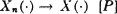
iffi there is a set E with P(E^c) = 0 such that X_n() → X() for each ∈ E.

Definition 6-3b

The sequence is said to converge almost uniformly to X(·), indicated

iffi, to each > 0, there corresponds a set E with P(E^c) < such that X_n() converges uniformly to X() for all ∈ .

Definition 6-3c

The sequence is said to converge in probability to X(·), indicated

iffi

Definition 6-3d

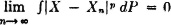
The sequence is said to converge in the mean of order p (p ≥ 1), indicated

iffi

Theorem 6-SD

Theorem 6-3E

If Y(·) is a nonnegative random variable such that Y^p(·) is integrable (p ≥ 1) and | X_n(·) | ≤ Y(·) [P], then, for p = 1, [P] ⇒ [a. unif], and for p ≥ 1, [in prob] ⇒ [mean^p], so that in this case

Theorem 6-3F

A sequence of random variables {X_n(·): 1 ≤ n < ∞} satisfies the condition

iffi

   (B) Each subsequence has a further subsequence which converges to X(·) with probability 1.

Expectations for random processes

Definition 7-6a

A process X is said to be of order p if, for each t ∈ T, E[|X(t)|^p] ≤ ∞ (p is a positive integer).

Definition 7-6b

The mean-value function for a process is the first moment

Definition 7-6e

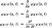
The covariance function K_X(·, ·) of a process X, if it exists, is the function defined by

The bar denotes the complex conjugate. The autocorrelation function _XX(·, ·) of a process, if it exists, is the function defined by

Definition 7-6f

The cross-correlation functions for two random processes X and Y are defined by

Properties of correlation functions

Definition 7-6g

A function g{·, ·) defined on T × T is positive semidefinite (or nonnegative definite) iffi, for every finite subset T_n contained in T and every function h(·) defined on T_n, it follows that

(1)

(2)

(3) The autocorrelation function _XX(·, ·) is positive semidefinite.

(4) The random process X is continuous [mean²] at t iffi the autocorrelation function _XX(·, ·) is continuous at the point t, t.

(5) If _XX(s, t) is continuous at all points t, t, it is continuous for all s, t.

(6) If exists for all points t, t, then X′(·, t) exists for all i.

(7) If X′(·, s) exists for all s and Y′(·, t) exists for all t, then the following correlation functions and partial derivatives exist and the equalities indicated hold:

Stationary random processes

Definition 7-7a

A random process X is said to be stationary iffi, for every choice of any finite number n of elements t₁, t₂, …, t_n from the parameter set T and of any h such that t₁ + h, t₂ + h, …, t_n + h all belong to T, we have the shift property F(·, t₁; ·, t₂) · · ·; ·, t_n) = F(·, t₁ + h; ·, t₂ + h; · · ·; ·, t_n + h)

Definition 7-7b

A random process X is said to be second-order stationary if it is of second order and if its first and second distribution functions have the shift property

If the process is of second order and _XX{t, t + τ) = _XX(0, τ) for all t, τ, the process is said to be stationary in the wide sense.