Chapter 9
Propeller Aircraft: Applied Performance

The aircraft performance items that we discussed in Chapter 8 were for one weight, clean configuration, and sea level standard day conditions. In this chapter we alter these conditions and examine the resulting performance for a change in weight, altitude, and configuration. To simplify the explanation, only one condition is altered at a time.

VARIATIONS IN THE POWER‐REQUIRED CURVE

The basic power‐required curve (Fig. 8.8) was drawn for a 20,000‐lb airplane in the clean configuration, at sea level on a standard day. We now show how the curve changes for variations in weight, configuration, and altitude.

Weight Changes

Weight change is inevitable on every flight; usually weight is reduced during a flight as fuel is consumed. As the mission changes, so do the operating parameters of each flight, so a pilot must be aware of how the aircraft's performance characteristics are going to change correspondingly. As weight is increased, the P_r to overcome the increase in drag due to the increase lift must also increase. As the power increases, so must the fuel flow and all related performance values.

To find out how the varies with weight changes, we go back to the basic relationship between and (drag) that we developed in Eq. 1.13:

Adding subscripts and forming a ratio gives

From Eq. 7.1,

And from Eq. 4.3,

Substituting gives

(9.1)

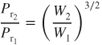
In addition to the increase in , with an increase in weight there also must be an increase in velocity. This is the same as was found in Eq. 4.3:

In plotting new curves for a change in weight, both Eqs. 9.1 and 4.3 must be applied. Figure 9.1 shows curves for 20,000 and 30,000 lb. As weight is decreased, the curve shifts down and to the left; all previous “V speeds” for endurance, specific range, and steady‐velocity climbs must shift as well.

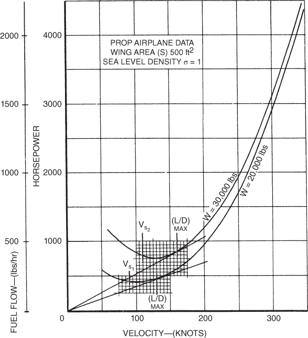
Figure 9.1 Effect of weight change on a curve.

Configuration Change

In going from the clean configuration to the gear and flaps down (dirty) configuration, the equivalent parasite area is greatly increased. For the airplane shown in Fig. 9.2, it increases by 50% (from 9.92 to 14.9 ft²). This increases the parasite drag, and thus the parasite power required, but has little effect on the induced drag or induced power required. As we have seen with a power‐producer, the faster the aircraft travels the more power must be produced to overcome the increased parasite drag, which means more fuel must be consumed per unit of time.

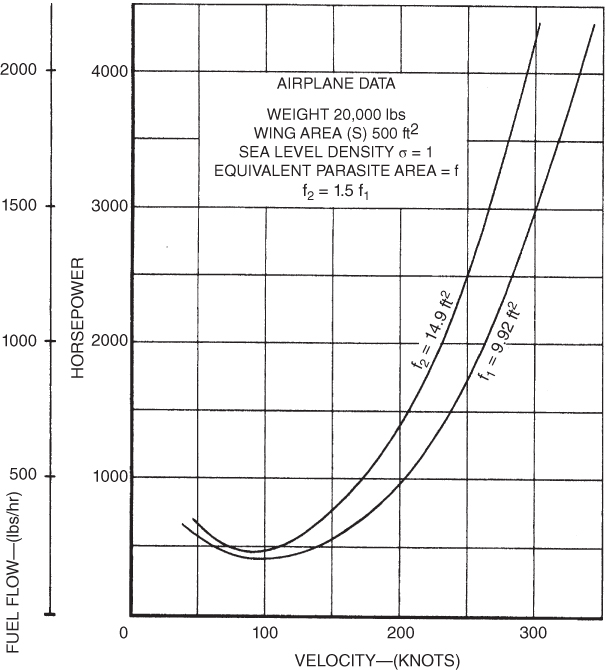
Figure 9.2 Effect of configuration on the curve.

There is no short‐cut method of calculating the curve for the dirty condition. You must calculate the parasite drag and then the total drag for the dirty condition, and then convert this to power required by Eq. 1.13. The effect of configuration change is shown on the curves in Fig. 9.2.

Altitude Changes

In our discussion of the effect of altitude on the drag of an aircraft, we saw that the drag of the aircraft was unaffected by altitude, but that the true airspeed at which the drag occurred did change:

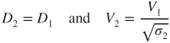
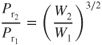
Subscript 1 is sea level () and subscript 2 is at altitude. Applying the above equations to Eq. 1.13 gives

(9.2)

The drag does not change with altitude but the does. The velocity changes by the same amount:

(9.3)

In plotting new curves for a change in altitude, note that both Eq. 9.2 and Eq. 9.3 must be applied. All points on the sea level curve move to the right and upward, by the same amount, when correcting for altitude changes. This is shown in Fig. 9.3. Note that the line drawn from the origin, which is tangent to the curve and locates the point, remains tangent to the curve at all altitudes. The angle remains the same at all altitudes. The significance of this is explained later in this chapter.

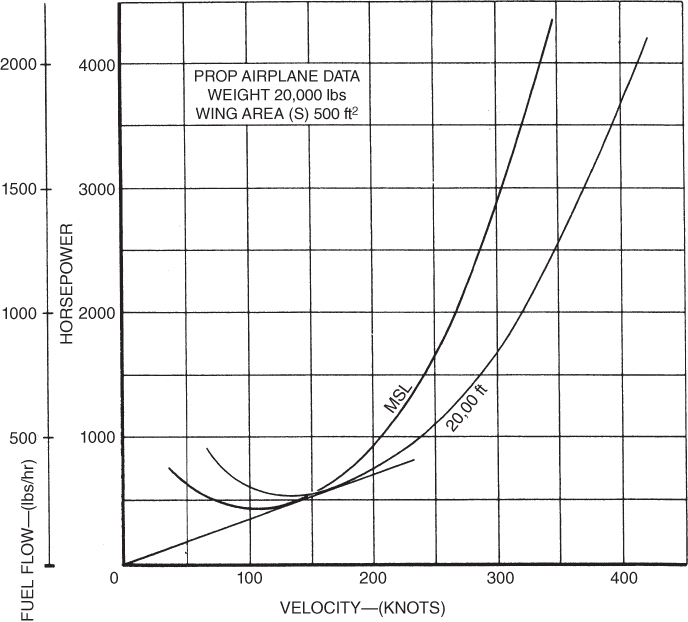
Figure 9.3 Effect of altitude on a curve.

Another point of interest in the altitude curves is that the curves move farther apart at higher velocities. Each point on the sea level curve is moved to the right and also moved upward by the same multiplier, , so the change is greater when the velocity or power required is greater; thus, points on the right are changed more than those on the left. Even though the drag at sea level is equal to the drag at altitude, proportionally greater power is required because of the higher true airspeed.

VARIATIONS IN AIRCRAFT PERFORMANCE

Straight and Level Flight

Weight Change

In straight and level, unaccelerated flight all forces are equal, so if weight is increased then so must the lift, which means so must the induced drag. To remain in level flight P_r increases to equalize the increase in drag, so an increase in weight means an increase in , but is not changed; is decreased. A reduction in weight has the opposite effect and will be increased.

Configuration Change

in the dirty configuration is usually limited by structural strength of gear and flaps, so is reduced. Since parasite drag increases as speed increases, and the power required to overcome the parasite drag also increases, decreases. As the gear and flaps are retracted, then parasite drag decreases for a given velocity, so now also decreases to maintain level flight and increases for a given .

Altitude Increase

The power available at altitude is affected by the type of engine and/or propeller. If turbocharged reciprocating engines with constant speed props are flown below their critical altitude they can develop as much power as at sea level. In this case the TAS will be increased significantly. Nonturbocharged reciprocating engines with fixed props, on the other hand, will suffer a power loss as altitude increases and may experience either an increase or a decrease in , depending on the intersection point of the and curves. Similar reasoning can be applied to turboprop engines. The engine loses power with increased altitude, but the curve moves to the right, so the intersection of the curves will determine . The IAS will be lower in all cases.

Climb Performance

As we have discussed, climb performance of a power‐producer depends on excess thrust for best angle of climb (), and excess power for best rate of climb (). As weight, configuration, and altitude change so do these climb performance characteristics. As altitude is increased for a given aircraft, the will increase and the will decrease. When the aircraft is unable to climb at a rate of 100 fpm, then the service ceiling has been reached. When the aircraft has no excess power and produces zero climb rate, absolute ceiling has been reached. Figure 9.4 is a standard plot of versus for a climb in standard altitude.

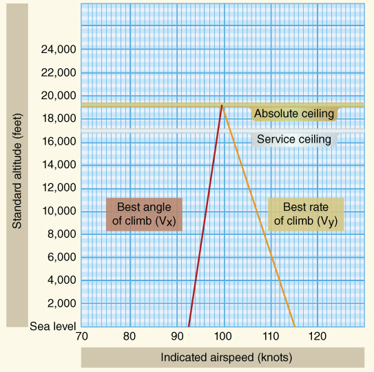
Figure 9.4 versus with altitude.

U.S. Department of Transportation Federal Aviation Administration, Pilot's Handbook of Aeronautical Knowledge, 2008

Angle of Climb

Weight Change

Increased weight results in increased power required, while power available is not changed. Equation 8.6 shows:

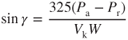
Both the excess power reduction and the increased weight cause a reduction in angle of climb.

Configuration Change

Power required increases in the dirty configuration due to the increase in total drag (mainly parasite drag); thus, the angle of climb is reduced. However, the increase in is much less than was the increase in for the jet aircraft (see Figs. 9.2 and 7.4). Again the superior performance, at low speeds, of propeller aircraft is demonstrated.

Altitude Increase

From Eq. 8.6, it can also be seen that the increase in at altitude will reduce the angle of climb, even if is not reduced.

Rate of Climb

Weight Change

As with angle of climb, when weight increases the drag increases due to the increase in lift required to compensate for the weight, must increase accordingly. Rate of climb is calculated by Eq. 8.7:

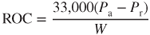
When the value of weight in the equation above increases, increases as remains the same, ROC must decrease. As weight decreases then the ROC increases as excess power is available.

Configuration Change

Dirty aircraft experience a reduction in rate of climb performance as with the angle of climb discussion above. In order to maximize the performance of an aircraft after takeoff, during missed approach in inclement weather, or in an emergency, retract the gear as soon as possible and retract the flaps as required.

Endurance

Weight Change

We have seen that more power is required with an increase in weight. Since fuel flow is proportional to , any increase in power required means a decrease in endurance. The opposite is true when weight is decreased: endurance is increased.

Configuration Change

Endurance is directly proportional to fuel flow; if drag is increased due to the deployment of gear and flaps, P_r increases and thus fuel flow increases. When in a holding pattern keep the gear retracted, deploy approach flaps as required, and slow down to reduce parasite drag.

Altitude Increase

With a turboprop, the reduction in fuel flow at altitude will more than compensate for the increase in but if it is necessary to climb to altitude, more fuel may be required than if the airplane had remained at the lower altitude. For a reciprocating engine, the endurance at altitude is reduced, but only if the fuel/air mixture is leaned appropriately. So be aware of the manufacturer's recommendations when manually adjusting the mixture.

Specific Range

Weight Change

As fuel is burned, weight is reduced, and the power‐required curve moves downward and to the left. This is shown in Fig. 9.5. The tangent lines intersect the curves at and indicate the maximum specific range velocity and fuel flow at this point. At a gross weight of 30,000 lb, the velocity must be 160 knots for maximum range and the fuel flow will be 425 lb/hr. The SR here is 160/425 = 0.3765 nmi/lb.

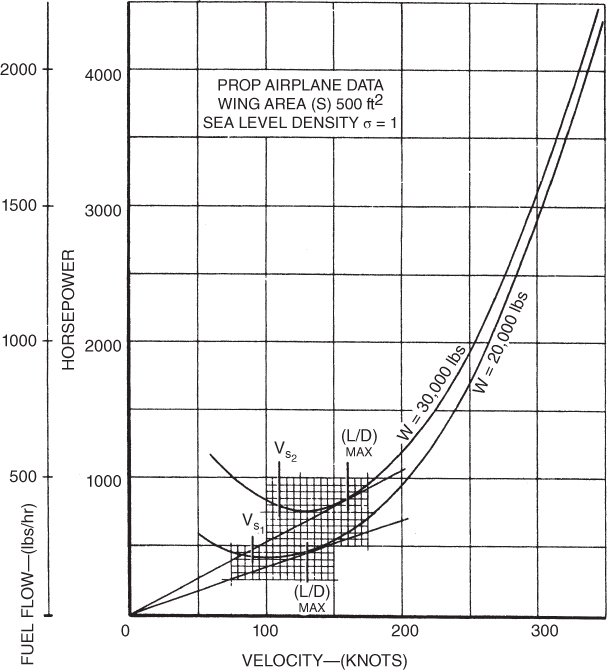
Figure 9.5 Effect of weight change on specific range.

When the weight of the aircraft has been reduced to 20,000 lb, the aircraft must fly at 130 knots to attain maximum range. The fuel flow here will be 225 lb/hr and the SR = 130/225 = 0.5778 nmi/lb. This is a 53.5% improvement in specific range. The pilot must reduce the power output of the engine and reduce the airspeed to achieve this range. It is only necessary for the pilot to reduce the power setting because the airspeed will automatically be reduced when this is done.

The natural tendency of a pilot is to keep the power setting the same, as fuel is burned, and to allow the velocity to increase as the drag decreases when fuel is consumed. This will not maintain the maximum range and will in fact reduce the range by an appreciable amount. For maximum range, as weight is reduced, reduce airspeed.

Configuration Change

If it is necessary to fly in the dirty configuration, slow the airplane to reduce drag, if the AOA is known for the new configuration then that AOA should be maintained.

Altitude Increase

In our earlier discussion we pointed out that an altitude increase changed both the and the velocity by the same amount. We also saw that the tangent line to the curves remained the same for all altitudes. In Fig. 8.18 we saw that the intersection of the tangent line and the curve indicated the maximum specific range point. Thus, as far as the airframe is concerned, the altitude has no effect on the specific range (Fig. 9.6). The ratio of fuel flow to velocity is constant with altitude. Propeller‐driven airplanes do not show large increases in range as jet airplanes do.

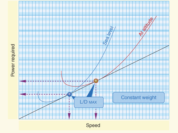
Figure 9.6 Effect of altitude on specific range.

U.S. Department of Transportation Federal Aviation Administration, Pilot's Handbook of Aeronautical Knowledge, 2008

We must consider at what altitude the engine–propeller combination is most efficient. First, let's look at the nonturbocharged reciprocating engine with a fixed‐pitch propeller. This engine can develop sea level power to about 5000 ft. This seems to be about the altitude where maximum range is obtained. For the turbocharged reciprocating engine with constant speed propeller, about 10,000 ft is best. The turbine engine of the turboprop aircraft likes high altitude and operates best at about 25,000 ft.

EQUATIONS

1. 9.1
2. 9.2
3. 9.3

PROBLEMS

1. A lightly loaded propeller airplane will be able to glide ______ when it is heavily loaded.
   1. farther than
   2. less far than
   3. the same distance as
2. To obtain maximum glide distance, a heavily loaded airplane must be flown at a higher airspeed than if it is lightly loaded.
   1. True
   2. False
3. In order to maximize range on a propeller‐driven airplane at high altitude, true airspeed should be
   1. decreased.
   2. increased.
   3. not changed.
4. In Fig. 9.3, the specific range for a propeller airplane is
   1. less at altitude than at sea level.
   2. more at altitude than at sea level.
   3. the same at altitude as at sea level.
5. The pilot of a propeller airplane is flying at the speed for best range under no‐wind conditions. A head wind is encountered. To obtain best range the pilot now must
   1. speed up by the amount of the wind speed.
   2. slow down by the amount of the wind speed.
   3. speed up by less than the wind speed.
   4. slow down by more than the wind speed.
6. As a propeller airplane burns up fuel, to fly for maximum range, the airspeed must
   1. remain the same.
   2. be allowed to speed up.
   3. be slowed down.
7. The turboprop aircraft has its lowest specific fuel consumption at about 25,000 ft altitude because
   1. the turbine engine wants to fly at high altitudes.
   2. the propeller has higher efficiency at lower altitudes.
   3. This is a compromise between (a) and (b) above.
8. The power‐required curves for an increase in altitude show that the
   1. remains the same as altitude increases.
   2. increases by the same amount as the velocity.
   3. increases but the velocity does not.
9. A propeller aircraft in the dirty condition shows that the moves up and to the left over the clean configuration. This is because
   1. the increase in the induced is more at low speed.
   2. the increase is mostly due to parasite .
   3. both induced and parasite increase by the same amount.
10. The increase in the curves for a weight increase is greater at low speeds than at high speeds because the increase in
    1. induced is greatest.
    2. parasite is greatest.
    3. profile is greatest.
11. Using Fig. 9.1, find the velocity for the best range for the airplane at 30,000 lb and 20,000 lb gross weight (GW).
12. Using Fig. 9.1, calculate the specific range for the airplane at both weights if it is flying at the best range airspeed.
13. Using Fig. 9.1. calculate the specific range for the 20,000‐lb airplane if the throttle is not retarded and the airspeed is allowed to increase as weight is reduced. Compare your answer to that of Problem 12 and state your conclusions.
14. Using Fig. 9.3, calculate the specific range for this airplane if it is flying at best range airspeed at mean sea level (MSL) and also at 20,000 ft altitude.
15. A 20,000‐lb propeller airplane at sea level standard day has the following data. Calculate its and plot the curve on the graph paper.

    V	Drag	Pr
    150	2074
    182.7	1923
    200	1954
    300	2948
    400	4809

16. The airplane in Problem 15 now has its gross weight increased to 30,000 lb. Calculate the new values and plot the curve on the graph paper.

    150
    182.7
    200
    300
    400

17. Calculate new values for the 20,000‐lb airplane in Problem 15, but now flying at 20,000 ft density altitude. Plot the values and draw the curve on the graph paper.

    150
    182.7
    200
    300
    400