Chapter 13
Maneuvering Performance

For our discussion, maneuvering performance will be divided into two main categories: general turning performance and energy maneuverability. General turning performance is common to all aircraft. It involves constant altitude turns and constant speed (but not constant velocity) conditions. Remember, velocity is a vector, having speed and direction. Energy maneuvering is relevant to tactical military missions, such as air‐to‐air combat maneuvers and air‐to‐ground maneuvers.

The discussion in this chapter does not cover energy maneuverability, but is confined to general turning flight and the flight envelope limitations on an aircraft.

GENERAL TURNING PERFORMANCE

In turning flight the airplane is not in a state of equilibrium, since there must be an unbalanced force to accelerate the plane into the turn. As the angle of bank increases in a level turn, so will the unbalanced force (Fig. 13.1). Unlike other vehicles, an airplane must be banked in order to turn, and to maintain level flight the AOA must be increased.

Figure 13.1 Increasing bank angle and related forces.

U.S. Department of Transportation Federal Aviation Administration, Pilot's Handbook of Aeronautical Knowledge, 2008

First, let us review acceleration. In Chapter 1 acceleration was defined as the change in velocity per unit of time. Velocity was defined as a vector quantity that involves both the speed of an object and the direction of the object's motion. Any change in the direction of a turning aircraft is therefore a change in its velocity, even though its speed remains constant. An aircraft in a turn is subjected to an unbalanced force acting toward the center of rotation. Newton's first law states that a body at rest will remain at rest, and a body in motion will remain in motion, in a straight line, unless acted on by an unbalanced force. Newton's second law then states that an unbalanced force will accelerate a body in the direction of that force. This unbalanced force is called the centripetal force, commonly referred to as the horizontal component of lift, and it produces an acceleration toward the center of rotation known as radial acceleration.

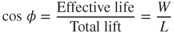
The forces acting on an aircraft in a coordinated, constant altitude turn are shown in Fig. 13.2. In wings level, constant altitude flight, the lift equals the weight of the airplane and is opposite to it in direction. But in turning flight, the lift is not opposite, in direction, to the weight. Only the vertical component of the lift, called effective lift, is available to offset the weight. Thus, if constant altitude is to be maintained, the total lift must be increased until the effective lift equals weight. An aircraft in a ∼45° bank, maintaining level flight, has roughly 80% of the original effective lift. Until the remaining 20% loss of vertical lift is replaced the aircraft will not be able to maintain level flight.

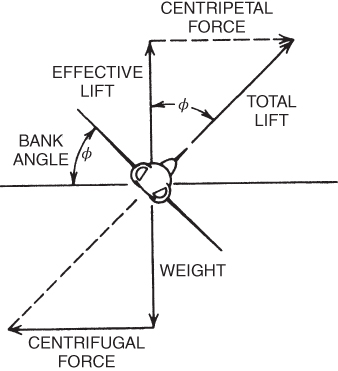
Figure 13.2 Forces on an aircraft in a coordinated level turn.

Solving the triangle in Fig. 13.2 gives

(13.1)

The load factor, G, on the aircraft is defined as the ratio of the maximum load an aircraft can sustain to the total weight of the aircraft, or lift/weight:

(13.2)

Inverting Eq. 13.1 and substituting the value of L/W into Eq. 13.2, we obtain

(13.3)

G is called the load factor. The centripetal force causing the airplane to turn is found by solving the triangle in triangle in Fig. 13.2:

So

(13.4)

The equal and opposite reaction force described in Newton's third law is called the centrifugal force. This force is the airplane's inertia, which resists the turn.

A vector diagram of the forces acting on an airplane in a coordinated constant altitude turn is shown in Fig. 13.3. From Eq. 13.2 it can be seen that the total lift, L, can be replaced by its equivalent, GW.

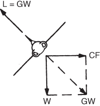
Figure 13.3 Vector diagram of forces on an aircraft in a turn.

Load Factors on an Aircraft in a Coordinated Turn

Understanding load factors and the ability of an aircraft (and pilot) to withstand +/‐ 1G flight is vital for safety of flight. Without this understanding a pilot may inadvertently overload the aircraft structure, damaging the aircraft, or worse. An increased load factor also increases the stall speed, and an accelerated stall may occur to an unsuspecting pilot at an airspeed much higher than V_S0.

Equation 13.3 tells us that the G's required for an aircraft to maintain altitude in a coordinated turn are determined by the bank angle alone. Type of aircraft, airspeed, or other factors have no influence on the load factor. Any aircraft maintaining level flight, in a 60° bank, will have a load factor of 2 Gs. If the total gross weight of the aircraft is 2500 lb, the wings must produce enough lift to sustain 5000 lb to maintain level flight. Figure 13.4 depicts the load factors required at various bank angles, note that above 45° the load factor increases at a much faster rate.

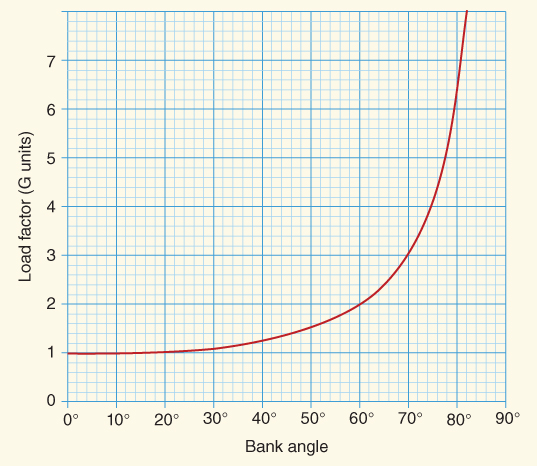
Figure 13.4 Load factors at various bank angles.

U.S. Department of Transportation Federal Aviation Administration, Pilot's Handbook of Aeronautical Knowledge, 2008

Note that the load factors required to fly at constant altitude in turning flight were determined by assuming that the wings of the aircraft provided all the lift of the aircraft. According to this analysis, the load factor at a 90° bank will be infinity and thus impossible to attain. But we have all seen aircraft fly an eight‐point roll, with the roll stopped at the 90° position. The secret is that lift is provided by parts of the aircraft other than the wings. If the nose of the aircraft is held above the horizontal, the vertical component of the thrust will act as lift. The fuselage is also operating at some effective AOA and will develop lift. The vertical tail and rudder will also develop lift.

Figure 13.5 shows the forces on an aircraft after it has rolled 90°. One of three possible limiting factors on turning performance is the structural strength limits of the airplane. We have just discussed this limitation. The bank angle determines the load factor and may limit the turn radius.

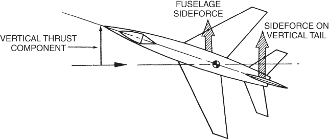
Figure 13.5 Forces on an aircraft during a 90° roll.

Effect of a Coordinated Banked Turn on Stall Speed

In basic aerodynamics we learned that the aircraft always develops its slow speed stall at the stall AOA. At this AOA the value of the lift coefficient is a maximum, C_L(max). So V_S occurs at C_L(max). The basic lift equation 4.2 can be rewritten as

and since L = GW,

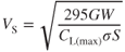
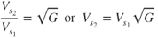
Thus, stall speed depends on the square root of the G loading. All other factors in the equation are constant for the same altitude. Therefore,

(13.5)

where

	=	stall speed under 1G flight
	=	stall speed under other than 1G flight
G	=	load factor for condition 2

Substituting the value of G from Eq 13.3. gives

(13.6)

Any aircraft can be stalled at any airspeed within its design limits. From Eq. 13.5 above, an aircraft with an unaccelerated stall speed of 50 kts, can be stalled at 100 kts if experiencing a load factor of 4 Gs. Pilots need to be aware that in a constant altitude, increasing bank turn, the stall speed is increasing and the indicated airspeed is decreasing (Fig. 13.6).

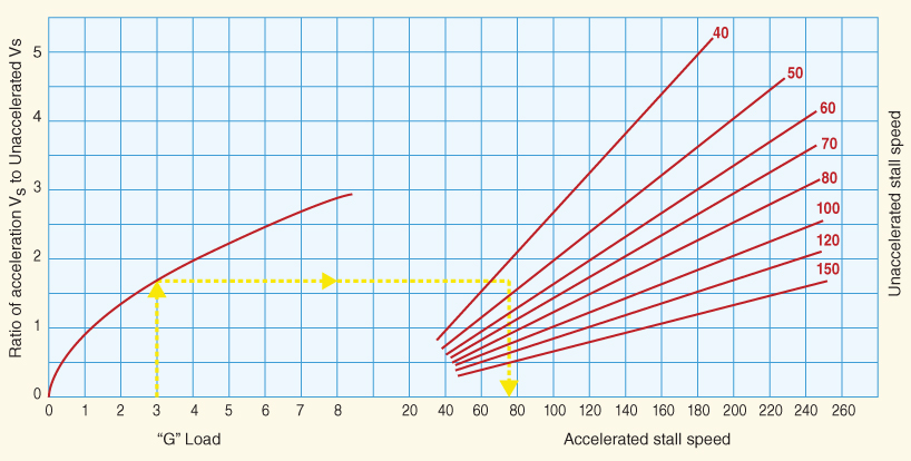
Figure 13.6 Load factor and stall speed.

U.S. Department of Transportation Federal Aviation Administration, Pilot's Handbook of Aeronautical Knowledge, 2008

The V–G Diagram (Flight Envelope)

Equation 13.5 shows how the stall speed increases as greater than 1G loading is applied to an aircraft. If an aircraft is under a 4G load, the stall speed is the square root of 4 or twice the 1G stall speed. At zero G the stall speed is zero because no lift is being developed. This equation cannot be applied when an aircraft is developing negative load factors (square root of a negative number is impossible), but an aircraft can be stalled under negative G loading.

Figure 13.7 shows the first construction lines of the V–G diagram (flight envelope), the plot of the stall speed at various G loadings. This velocity versus G load diagram is valid for a certain aircraft, with a given weight and altitude. These curved lines can also be thought of as the number of Gs that can be applied to the aircraft before it will stall at a given airspeed. They are called the aerodynamic limits of the aircraft. It is impossible to fly to the left of these curves, because the aircraft is stalled in this region.

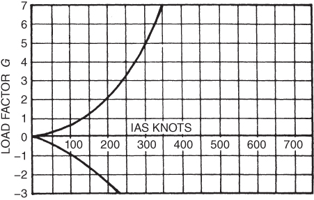
Figure 13.7 First‐stage construction of a V–G diagram.

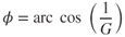
Equation 13.3 relates the G loading to the bank angle. Rearranging this equation we see that the bank angle is the angle whose cosine is 1/G. Mathematically, this is

(13.7)

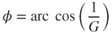
Table 13.1 shows the bank angles that produce the load factors shown in Fig. 13.7.

Table 13.1 Load Factors at Various Bank Angles

Load Factor, G	Bank Angle, θ°
1	0
2	60
3	70.5
4	75.5
5	78.5
6	80.4
7	81.8

The second stage of construction of the V–G diagram consists of drawing horizontal lines at the positive and negative limit load factors, LLFs. These limits are specified for each model aircraft and are shown in Fig. 13.8 as limit load factor +7G and as limit load factor −3G. The Federal Aviation Administration (FAA) has designed a category system for many general aviation aircraft, a placard in the flight deck as well as warnings in the Airplane Flight Manual (AFM) specify what category (or categories) that aircraft may be operated which apply to the following LLFs:

• Normal Category ‐ +3.8 to −1.52
• Utility Category ‐ +4.4 to −1.76
• Acrobatic Category ‐ +6.0 to −3.00

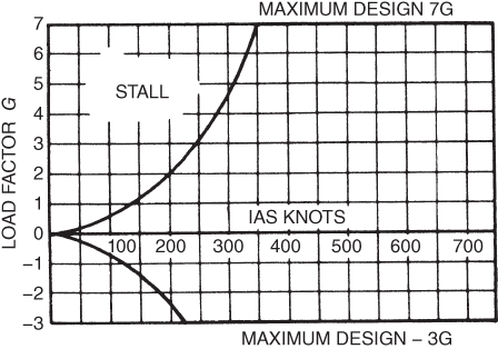
Figure 13.8 Second‐stage construction of V–G diagram.

The structural limit load factors show the maximum G's that may be imposed on the aircraft in flight without damaging the structure. Pilots should be aware of the load factors they are imposing on the aircraft at all times; accidents involving stalls initiated from steep turns in addition to structural failures as the result of poorly executed acrobatics may occur. With experience a pilot may be able to judge the amount of load factor imposed on an aircraft, more accurate measures can be determined by installing an accelerometer, though these are rare within general aviation.

Several important facts about load factors should be understood: First, the limits are for a certain gross weight, and they change if the gross weight differs from that specified. Second, the limits are for symmetrical loading only. Third, the assumption is made that there is no corrosion, metal fatigue or other damage to the aircraft. Fourth, up‐gusts and turbulent air can add to pilot imposed load factors.

The aircraft designer designs a certain strength into the airframe. The allowable total strength divided by the weight of the aircraft determines the limit load factor. If the design weight is exceeded, then the number of G's that can be tolerated by the airframe must decrease. This is an inverse proportion:

(13.8)

During unsymmetrical maneuvers, such as a rolling pullout, the wing that is rising will have more lift on it, and thus a greater load factor, than the down‐going wing. This is shown in Fig. 13.9. The accelerometer is located on the center line of the aircraft and will measure the average load factor. In Fig. 13.9, the pilot reads 5Gs, but the up‐going wing will actually be subjected to 7G's.

Figure 13.9 Antisymmetrical loading.

Maneuver Speed

An interesting point on the V–G diagram is the intersection of the aerodynamic limit line and the structural limit line. The aircraft's speed at this point is called the maneuver speed, V_A, commonly called corner speed. All pilots need to be aware of what this speed is for their airplane on a given day. V_A is usually published in the AFM as well as placarded on the instrument panel for maximum visibility, and is usually the maneuver speed at the maximum gross weight. As the weight of the aircraft decreases, so will V_A.

At any speed below the maneuver speed the aircraft cannot be overstressed; it will stall before the limit load factor is reached. Above this speed, however, the aircraft can exceed the limit load factor before it stalls. At the maneuver airspeed the aircraft's limit load factor will be reached at the lowest possible airspeed.

Performing acrobatic maneuvers and steeply banked turns are not the only time the importance of V_A should be noted, when entering turbulent air an aircraft should be slowed to an airspeed below V_A. Due to gust factors and unexpected turbulence, especially around thunderstorms and when crossing fronts, adherence to design maneuvering speed is imperative. Clear air turbulence, often close to the tropopause or jetstream, but not uncommon down to 15,000 ft, also may lead to turbulent air resulting in a reduction in speed below V_A.

The maneuver airspeed, V_A, is shown in Fig. 13.10. It can be calculated by

(13.9)

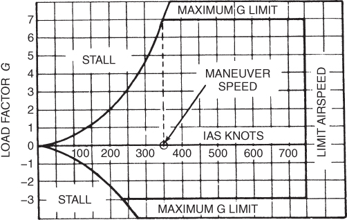
Figure 13.10 Maneuver (corner) speed.

where

VA	=	maneuver speed (knots)
VS	=	stall speed (knots)
LLF	=	limit load factor

All missions that an aircraft is designed to perform can be accomplished without exceeding the limit load factors, but on occasion a pilot will cause the aircraft to exceed these load factors. If this happens, the aircraft will probably suffer permanent objectionable deformation (aircraft components do not return to their original shape), resulting in costly repairs, but it will not necessarily result in failure of the primary structure.

There is another load factor that, if exceeded, may lead to catastrophic failure of the airframe. This load factor is called the ultimate load factor, ULF. Numerically the positive and negative ultimate load factors are 1.5 times the limit load factors. These are shown in Fig. 13.11 and are labeled as structural failure.

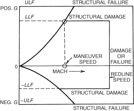
Figure 13.11 Ultimate load factors.

The high‐speed limit of the V–G diagram is called the never exceed velocity, V_NE, or, more commonly, the redline speed. It is shown in Fig. 13.11. If the redline speed is exceeded structural failure may occur.

The pilot must stay inside of the flight envelope or the airplane will be in the structural damage or structural failure area.

Radius of Turn

The radius of a turn is very important depending on the mission of the flight, as in air‐to‐air combat, or in an escape situation as when exiting a box canyon. As we have discussed, increased bank angle during a coordinated turn in level flight decreases the turn radius. When an aircraft increases its bank angle to limit the turn radius, stall speed increases. A balance must be found between the necessary bank angle to achieve air superiority or successful terrain avoidance, while at the same time maintaining a safe margin above stall speed without exceeding V_A. Figure 13.12 shows the varying bank angle, stall speed, and turn radius for a glider attempting to remain in a thermal.

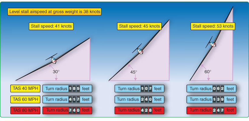
Figure 13.12 Stall speed and turn radius with varying angle of bank.

U.S. Department of Transportation Federal Aviation Administration, Glider Flying Handbook, 2013

The radius of a turn and rate of a turn are directly linked. Figure 13.13 shows that the radius of a turn increases in two situations, constant angle of bank with increasing airspeed, and constant airspeed with decreasing angle of bank. The radius of a turn decreases when the situations are reversed.

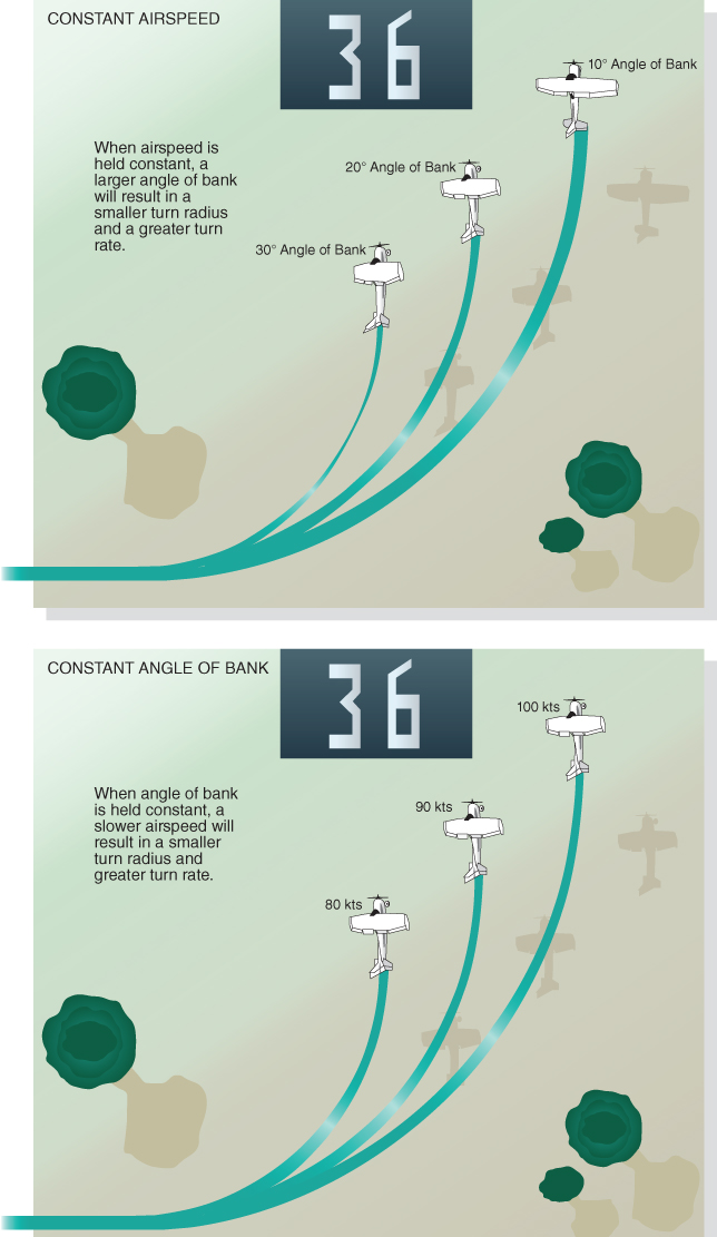
Figure 13.13 Rate and radius of a turn.

U.S. Department of Transportation Federal Aviation Administration, Airplane Flying Handbook, 2004

A body traveling in a circular path is undergoing an acceleration toward the center of rotation. This is called radial acceleration, a_r. It is a function of the velocity of the body, V, and the radius, r, of the circle:

(13.10)

As was shown in Fig. 13.2, the horizontal component of the total lift is the centripetal force that causes the radial acceleration. Also, the reaction force to the centripetal force, called the centrifugal force (CF), is equal in magnitude and opposite in direction to the centripetal force. The centripetal force in an automobile making a turn is generated by the friction of the car's tires on the pavement. The force that pulls the driver outward, away from the center of the turn, is the centrifugal force.

Since the centrifugal force is equal to the centripetal force in magnitude and results from the radial acceleration, it is, according to Newton's second law, equal to the mass times the radial acceleration:

(13.11)

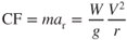
Equation 14.4 showed that this force is

Equating CF values gives

(13.12)

Equation 14.1 then can be rewritten as

(13.13)

By dividing Eq. 13.12 by Eq. 13.13 we obtain

(13.14)

This is the radius of turn equation.

Equation 13.14 was derived in basic units, and thus the velocity is in units of feet per second. If V is measured in knots, then

(13.15)

where

r	=	radius of turn (ft)
Vk	=	velocity (knots TAS)
φ	=	bank angle (degrees)

Rate of Turn

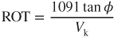
The rate of turn, ROT, is primarily used during instrument flight, and is the change in heading of the aircraft per unit of time:

If velocity is in knots and ROT is measured in degrees per second, then

(13.16)

A standard rate turn is considered to be 3°/sec, and depending on the TAS is the normal rate of turn for a general aviation aircraft operating in IMC. Faster aircraft often turn at a slower rate of 1.5°/sec due to the increased bank angle if a normal 3°/sec were to be maintained. A rough approximation of the angle of bank can be determined by dividing the TAS (knots) by 10 and then adding 5, so with a TAS of 110 kts the bank angle is ∼16°.

The importance of bank angle and velocity can be seen in Eqs. 13.15 and 13.16. High bank angles and slower airspeeds produce small turn radii and high ROT. Figure 13.13 once again shows us the relationship of ROT and bank angle. ROT decreases when a constant airspeed is maintained and angle of bank increases, or airspeed is decreased while maintaining a constant angle of bank. As before, the ROT increases when the situations are reversed.

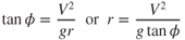
The maneuver speed is the speed at which highest bank angle can be achieved at minimum airspeed. Minimum turn radius and maximum rate of turn will be realized at this speed. Figure 13.14 is a chart that shows turn radii and rates of turn for various bank angles and airspeeds for an aircraft making a coordinated, constant altitude turn.

Figure 13.14 Constant altitude turn performance.

In our discussion of induced drag in Chapter 5 we saw that the rearward component of the total lift vector was induced drag and that the vertical component was effective lift. These are shown in Fig. 13.15. We see that the effective lift must equal the weight of the plane if constant altitude is to be maintained. We also see that more thrust is required to overcome this increase in induced drag, if airspeed is to be maintained. Thus, it may be that the turn radius may be limited by thrust available instead of structural limitations.

Figure 13.15 Forces on the complete aircraft.

Figure 13.16 shows a thrust‐limited aircraft's turn radius plotted against true airspeed. The aerodynamic limits are the same as were described for Fig. 13.10. The thrust limit curve is determined by a combination of bank angle and airspeed.

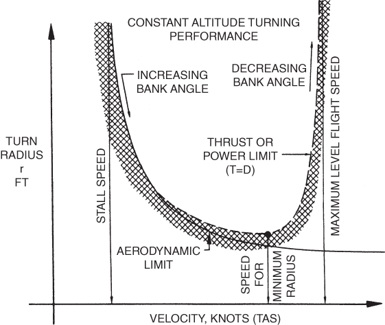
Figure 13.16 Thrust‐limited turn radius.

Vertical Loop

The loop has little tactile value but is taught as a confidence maneuver. In theory a perfect loop is performed without a change in airspeed, but in practice this is seldom, if ever, achieved. The perfect loop is an exact vertical circle and would require a thrust/weight ratio greater than 1.0 to maintain constant airspeed during the climb portion of the loop. The airplane would also need large speed braking devices to enable it to maintain constant airspeed duringthe last half of the maneuver. In addition, extensive throttle “jockeying” would be required.

The perfect loop and a normal loop are shown in Fig. 13.17. The loop does not seem to fit into either of the two categories of maneuverability (general turning performance or energy maneuverability). Instead, it is somewhere in between.

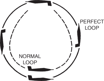
Figure 13.17 Perfect and normal loop.

The centrifugal force on the airplane depends on the weight, airspeed, and loop radius and can be calculated by use of Eq. 13.11:

The centrifugal force, CF, acts radially away from the center of the loop and is constant throughout the entire loop:

This is shown in Fig. 13.18. The G loading applied by the centrifugal forces alone is

(13.17)

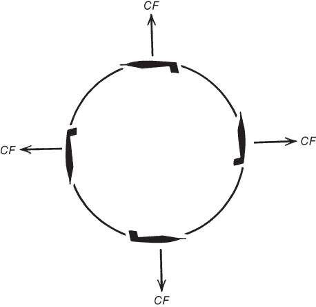
Figure 13.18 Centrifugal forces in a vertical loop.

---

Example

An aircraft flying at 296 knots (50 fps) and having a loop radius of 2604 ft experiences a centrifugal force of 3G's. The weight of the aircraft acting toward the earth also affects the G loading. The total Gs on the aircraft vary as the aircraft's altitude changes. Maximum Gs are and act at the bottom of the loop when the weight and centrifugal force act in the same direction.

At the top of the loop the aircraft is inverted, and the weight acts away from the centrifugal force. Gs at the top are . At the three and nine o'clock positions the weight does not affect the loading of the aircraft and . These load factors are shown in Fig. 13.19.

Figure 13.19 Loading on an example aircraft.

Actual Gs depend on airspeed and loop radius. However, the loss of 2G as an aircraft moves from the bottom of the loop to the top and the increase of 2Gs as the aircraft moves from the top to the bottom will hold true no matter what the applied G's are.

---

EQUATIONS

1. 13.1
2. 13.2
3. 13.3
4. 13.4
5. 13.5
6. 13.6
7. 13.7
8. 13.8
9. 13.9
10. 13.10
11. 13.11
12. 13.12
13. 13.13
14. 13.14
15. 13.15
16. 13.16
17. 13.17

PROBLEMS

1. In a constant altitude, constant airspeed turn, an aircraft is in a state of equilibrium.
   1. True
   2. False
2. The G forces on an airplane in a constant altitude turn depend on
   1. airspeed.
   2. type of airplane (jet or prop).
   3. bank angle.
   4. All of the above
3. An airplane performing an 8‐point roll can stop in the 90 position because
   1. the wings are not supporting the weight.
   2. the fuselage and vertical tail are supporting much of the weight.
   3. the pilot pulls the nose above the horizontal, thus some of the thrust helps support the weight.
   4. All of the above
4. When an airplane is in a constant altitude bank the stall speed
   1. remains the same as in level flight.
   2. increases as the square root of the G's.
   3. increases as the square root of 1/cos φ.
   4. Both (b) and (c)
5. What can we find from the aerodynamic limit line on a V − G diagram?
   1. It shows the maximum Gs that can be pulled at any airspeed below the corner speed.
   2. It shows the stall speed when Gs are being pulled.
   3. It is impossible to fly to the left of this line because the airplane will stall there.
   4. All of the above
6. The limit load factor (LLF) is also called maximum design G.
   1. True
   2. False
7. If the weight of an airplane. W₂, is increased above the design gross weight, W₁, the limit load factor
   1. remains the same.
   2. increases by the weight ratio, W₁/W₂.
   3. decreases by the weight ratio, W₁/W₂.
   4. None of the above
8. If an airplane is flying in symmetrical flight at its maneuver speed
   1. it cannot be overstressed.
   2. it can make the smallest turn radius.
   3. it can make the highest rate of turn.
   4. All of the above
9. The constant altitude turn performance chart (Fig. 13.14)
   1. can be used for only one particular model of airplane.
   2. does not show if the airplane is overstressed.
   3. is good for any model airplane.
   4. Both (b) and (c)
10. When an airplane makes a level banked turn, the airspeed will decrease (unless throttle is added), because
    1. parasite drag is increased the most.
    2. induced drag is increased the most.
    3. profile drag is increased the most.
11. A twin‐engine airplane has an engine failure shortly after takeoff. The pilot tries to turn back toward the field by making a left turn but crashes after making a 180° turn. The wreckage diagram shows that the turn radius was 6000 ft. The airspeed during the turn is estimated to be 200 knots TAS. Calculate the bank angle of the airplane.
12. Using Fig. 13.14 verify the answer to Problem 11.
13. Assuming a level turn, find the Gs on the airplane in Problem 11 during the turn.
14. For the airplane in Problem 11, calculate the rate of turn and time to make the 180 turn.
15. Using Fig. 13.14 verify the ROT you calculated in Problem 14.