Chapter 3
Formulas and Functions for Crunching Numbers
IN THIS CHAPTER
 Constructing a formula
Copying formulas to other columns and rows
Preventing errors in formulas
Using functions in formulas
Formulas are where it’s at as far as Excel is concerned. After you know how to construct formulas, and constructing them is pretty easy, you can put Excel to work. You can make the numbers speak to you. You can turn a bunch of unruly numbers into meaningful figures and statistics.
This chapter explains what a formula is, how to enter a formula, and how to enter a formula quickly. You also discover how to copy formulas from cell to cell and how to keep formula errors from creeping into your workbooks. Finally, this chapter explains how to make use of the hundred or so functions that Excel offers.
How Formulas Work
A formula, you may recall from the sleepy hours you spent in math class, is a way to calculate numbers. For example, 2+3=5 is a formula. When you enter a formula in a cell, Excel computes the formula and displays its results in the cell. Click in cell A3 and enter =2+3, for example, and Excel displays the number 5 in cell A3.
Referring to cells in formulas
As well as numbers, Excel formulas can refer to the contents of different cells. When a formula refers to a cell, the number in the cell is used to compute the formula. In Figure 3-1, for example, cell A1 contains the number 2; cell A2 contains the number 3; and cell A3 contains the formula =A1+A2. As shown in cell A3, the result of the formula is 5. If I change the number in cell A1 from 2 to 3, the result of the formula in cell A3 (=A1+A2) becomes 6, not 5. When a formula refers to a cell and the number in the cell changes, the result of the formula changes as well.
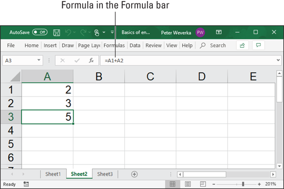
FIGURE 3-1: A simple formula.
To see the value of using cell references in formulas, consider the worksheet shown in Figure 3-2. The purpose of this worksheet is to track the budget of a school's Parent Teacher Association (PTA):
- Column C, Actual Income, lists income from different sources.
- Column D, Projected Income, shows what the PTA members thought income from these sources would be.
- Column E, Over/Under Budget, shows how actual income compares to projected income from the different sources.

FIGURE 3-2: Using formulas in a worksheet.
As the figures in the Actual Income column (column C) are updated, figures in the Over/Under Budget column (column E) and the Total Income row (row 8) change instantaneously. These figures change instantaneously because the formulas refer to the numbers in cells, not to unchanging numbers (known as constants).
Figure 3-3 shows the formulas used to calculate the data in the worksheet in Figure 3-2. In column E, formulas deduct the numbers in column D from the numbers in column C to show where the PTA over- or under-budgeted for the different sources of income. In row 8, you can see how the SUM function is used to total cells in rows 3 through 7. The end of this chapter explains how to use functions in formulas.
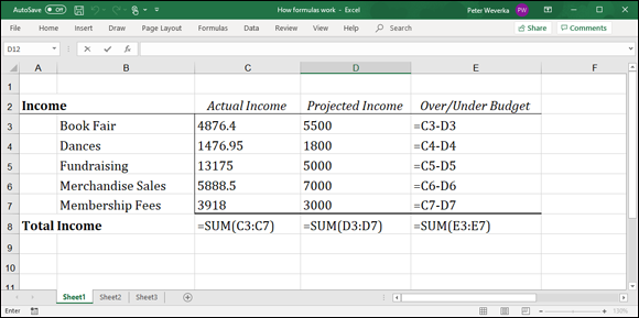
FIGURE 3-3: The formulas used to generate the numbers in Figure 3-2.
 Excel is remarkably good about updating cell references in formulas when you move cells. To see how good Excel is, consider what happens to cell addresses in formulas when you delete a row in a worksheet. If a formula refers to cell C1 but you delete row B, row C becomes row B and the value in cell C1 changes addresses from C1 to B1. You would think that references in formulas to cell C1 would be out of date, but you would be wrong. Excel automatically adjusts all formulas that refer to cell C1. Those formulas now refer to cell B1 instead.
In case you’re curious, you can display formulas in worksheet cells instead of the results of formulas, as was done in Figure 3-3, by pressing Ctrl+’ (apostrophe) or clicking the Show Formulas button on the Formulas tab. (You may have to click the Formula Auditing button first, depending on the size of your screen.) Click the Show Formulas button a second time to see formula results again.
Referring to formula results in formulas
Besides referring to cells with numbers in them, you can refer to formula results in a cell. Consider the worksheet shown in Figure 3-4. The purpose of this worksheet is to track scoring by the players on a basketball team over three games:
- The Totals column (column E) shows the total points each player scored in the three games.
- The Average column (column F), using the formula results in the Totals column, determines how much each player has scored on average. The Average column does that by dividing the results in column E by 3, the number of games played.

FIGURE 3-4: Using formula results as other formulas.
In this case, Excel uses the results of the total-calculation formulas in column E to compute average points per game in column F.
Operators in formulas
Addition, subtraction, and division aren’t the only operators you can use in formulas. Table 3-1 explains the arithmetic operators you can use and the key you press to enter each operator. In the table, operators are listed in the order of precedence (see the “The order of precedence” sidebar for an explanation of precedence).
TABLE 3-1 Arithmetic Operators for Use in Formulas
Precedence |
Operator |
Example Formula |
Returns |
1 |
% (Percent) |
|
50 percent, or 0.5 |
2 |
^ (Exponentiation) |
|
50 to the second power, or 2500 |
3 |
* (Multiplication) |
|
The value in cell E2 multiplied by 4 |
3 |
/ (Division) |
|
The value in cell E2 divided by 3 |
4 |
+ (Addition) |
|
The sum of the values in those cells |
4 |
– (Subtraction) |
|
The value in cell G5 minus 8 |
5 |
& (Concatenation) |
|
The text Part No. and the value in cell D4 |
6 |
= (Equal to) |
|
If the value in cell C5 is equal to 4, returns |
6 |
<> (Not equal to) |
|
If the value in cell F3 is not equal to 9, returns |
6 |
< (Less than) |
|
If the value in cell B9 is less than the value in cell E11, returns |
6 |
<= (Less than or equal to) |
|
If the value in cell A4 is less than or equal to 9, returns |
6 |
> (Greater than) |
|
If the value in cell E8 is greater than 14, returns |
6 |
>= (Greater than or equal to) |
|
If the value in cell C3 is greater than or equal to the value in cell D3, returns |
Another way to compute a formula is to make use of a function. As “Working with Functions” explains, later in this chapter, a function is a built-in formula that comes with Excel. SUM, for example, adds the numbers in cells. AVERAGE finds the average of different numbers.
The Basics of Entering a Formula
No matter what kind of formula you enter, and no matter how complex the formula is, follow these basic steps to enter it:
- Click the cell where you want to enter the formula.
- Click in the Formula bar if you want to enter the data there rather than the cell.
Enter the equals sign (=).
You must be sure to enter the equals sign before you enter a formula. Without it, Excel thinks you're entering text or a number, not a formula.Enter the formula.
For example, enter =B1*.06. Make sure that you enter all cell addresses correctly. By the way, you can enter lowercase letters in cell references. Excel changes them to uppercase after you finish entering the formula. The next section in this chapter explains how to enter cell addresses quickly in formulas.
Press Enter or click the Enter button (the check mark on the Formula bar).
The result of the formula appears in the cell.
Speed Techniques for Entering Formulas
Entering formulas and making sure that all cell references are correct is a tedious activity, but fortunately for you, Excel offers a few techniques to make entering formulas easier. Read on to find out how ranges make entering cell references easier and how you can enter cell references in formulas by pointing and clicking. You also find instructions here for copying formulas.
Clicking cells to enter cell references
The hardest part about entering a formula is entering the cell references correctly. You have to squint to see which row and column the cell you want to refer to is in. You have to carefully type the right column letter and row number. However, instead of typing a cell reference, you can click the cell you want to refer to in a formula.
In the course of entering a formula, simply click the cell on your worksheet that you want to reference. As shown in Figure 3-5, shimmering marquee lights appear around the cell that you clicked so that you can clearly see which cell you’re referring to. The cell’s reference address, meanwhile, appears in the Formula bar. In Figure 3-5, I clicked cell F3 instead of entering its reference address on the Formula bar. The reference F3 appears on the Formula bar, and the marquee lights appear around cell F3.

FIGURE 3-5: Clicking to enter a cell reference.
Get in the habit of pointing and clicking cells to enter cell references in formulas. Clicking cells is easier than typing cell addresses, and the cell references are entered more accurately.
Entering a cell range
A cell range is a line or block of cells in a worksheet. Instead of typing cell reference addresses one at a time, you can simply select cells on your worksheet. In Figure 3-6, I selected cells C3, D3, E3, and F3 to form cell range C3:F3. This spares me the trouble of entering one at a time the cell addresses that I want in the range. The formula in Figure 3-6 uses the SUM function to total the numeric values in cell range C3:F3. Notice the marquee lights around the range C3:F3. The lights show precisely which range you’re selecting. Cell ranges come in especially handy where functions are concerned (see “Working with Functions,” later in this chapter).
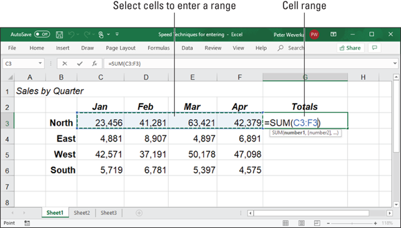
FIGURE 3-6: Using a cell range in a formula.
To identify a cell range, Excel lists the outermost cells in the range and places a colon (:) between cell addresses:
- A cell range comprising cells A1, A2, A3, and A4 is listed this way: A1:A4.
- A cell range comprising a block of cells from A1 to D4 is listed this way: A1:D4.
You can enter cell ranges on your own without selecting cells. To do so, type the first cell in the range, enter a colon (:), and type the last cell.
Naming cell ranges so that you can use them in formulas
Whether you type cell addresses yourself or drag across cells to enter a cell range, entering cell address references is a chore. Entering =C1+C2+C3+C4, for example, can cause a finger cramp; entering =SUM(C1:C4) is no piece of cake, either.
To take the tedium out of entering cell ranges in formulas, you can name cell ranges. Then, to enter a cell range in a formula, all you have to do is select a name in the Paste Name dialog box or click the Use in Formula button on the Formulas tab, as shown in Figure 3-7. Naming cell ranges has an added benefit: You can choose a name from the Name Box drop-down list and go directly to the cell range whose name you choose, as shown in Figure 3-7.
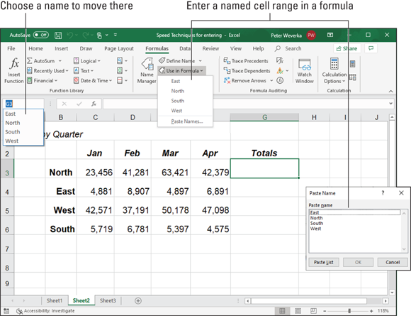
FIGURE 3-7: Choosing a named cell range.
 Naming cell ranges has one disadvantage, and it’s a big one. Excel doesn’t adjust cell references when you copy a formula with a range name from one cell to another. A range name always refers to the same set of cells. Later in this chapter, “Copying Formulas from Cell to Cell” explains how to copy formulas.
Creating a cell range name
Follow these steps to create a cell range name:
- Select the cells that you want to name.
On the Formulas tab, click the Define Name button.
You see the New Name dialog box.
Enter a descriptive name in the Name box.
Names can’t begin with a number or include blank spaces.
On the Scope drop-down list, choose Workbook or a worksheet name.
Choose a worksheet name if you intend to use the range name you’re creating only in formulas that you construct in a single worksheet. If your formulas will refer to cell range addresses in different worksheets, choose Workbook so that you can use the range name wherever you go in your workbook.
Enter a comment to describe the range name, if you want.
Enter a comment if doing so will help you remember where the cells you’re naming are located or what type of information they hold. As I explain shortly, you can read comments in the Name Manager dialog box, the place where you go to edit and delete range names.
- Click OK.
 In case you’re in a hurry, here’s a fast way to enter a cell range name: Select the cells for the range, click in the Name Box (you can find it on the left side of the Formula bar, as shown in Figure 3-7), enter a name for the range, and press the Enter key.
Entering a range name as part of a formula
To include a cell range name in a formula, click in the Formula bar where you want to enter the range name and then use one of these techniques to enter the name:
- On the Formulas tab, click the Use in Formula button and choose a cell range name on the drop-down list (refer to Figure 3-7).
- Press F3 or click the Use in Formula button and choose Paste Names on the drop-down list. You see the Paste Name dialog box (refer to Figure 3-7). Select a cell range name and click OK.
Quickly traveling to a cell range that you named
To go quickly to a cell range you named, open the drop-down list on the Name Box and choose a name (refer to Figure 3-7). The Name Box drop-down list is located on the left side of the Formula bar.
To make this trick work, the cursor can’t be in the Formula bar. The Name Box drop-down list isn’t available when you’re constructing a formula.
Managing cell range names
To rename, edit, or delete cell range names, go to the Formulas tab and click the Name Manager button. You see the Name Manager dialog box, as shown in Figure 3-8. This dialog box lists names, cell values in names, the worksheet on which the range name is found, and whether the range name can be applied throughout a workbook or only in one worksheet. To rename, edit, or delete a cell range name, select it in the dialog box and use these techniques:
- Renaming: Click the Edit button and enter a new name in the Edit Name dialog box.
- Reassigning cells: To assign different cells to a range name, click the Edit button. You see the Edit Name dialog box. To enter a new range of cells, either enter the cells’ addresses in the Refers To text box or click the Range Selector button (it’s to the right of the text box), drag across the cells on your worksheet that you want for the cell range, and click the Cell Selector button again to return to the Edit Name dialog box.
- Deleting: Click the Delete button and click OK in the confirmation box.
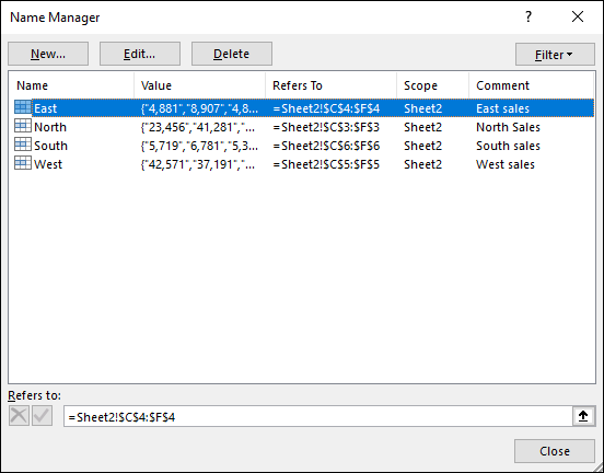
FIGURE 3-8: The Name Manager dialog box.
Referring to cells in different worksheets
Excel gives you the opportunity to use data from different worksheets in a formula. If one worksheet lists sales figures from January and the next lists sales figures from February, you can construct a “grand total” formula in either worksheet to tabulate sales in the two-month period. A reference to a cell on a different worksheet is called a 3D reference.
Construct the formula as you normally would, but when you want to refer to a cell or cell range in a different worksheet, click a worksheet tab to move to the other worksheet and select the cell or range of cells there. Without returning to the original worksheet, complete your formula in the Formula bar and press Enter. Excel returns you to the original worksheet, where you can see the results of your formula.
The only odd thing about constructing formulas across worksheets is the cell references. As a glance at the Formula bar tells you, cell addresses in cross-worksheet formulas list the sheet name and an exclamation point (!) as well as the cell address itself. For example, this formula in Sheet 1 adds the number in cell A4 to the numbers in cells D5 and E5 in Sheet 2:
=A4+Sheet2!D5+Sheet2!E5
This formula in Sheet 2 multiplies the number in cell E18 by the number in cell C15 in Worksheet 1:
=E18*Sheet1!C15
This formula in Sheet 2 finds the average of the numbers in the cell range C7:F7 in Sheet 1:
=AVERAGE(Sheet1!C7:F7)
Copying Formulas from Cell to Cell
Often in worksheets, you use the same formula across a row or down a column, but different cell references are used. For example, in the worksheet shown in Figure 3-9, column F totals the rainfall figures in rows 7 through 11. To enter formulas for totaling the rainfall figures in column F, you could laboriously enter formulas in cells F7, F8, F9, F10, and F11. But a faster way is to enter the formula once in cell F7 and then copy the formula in F7 down the column to cells F8, F9, F10, and F11.

FIGURE 3-9: Copying a formula.
When you copy a formula to a new cell, Excel adjusts the cell references in the formula so that the formula works in the cells to which it has been copied. Astounding! Opportunities to copy formulas abound on most worksheets. And copying formulas is the fastest and safest way to enter formulas in a worksheet.
Follow these steps to copy a formula:
- Select the cell with the formula you want to copy down a column or across a row.
Drag the AutoFill handle across the cells to which you want to copy the formula.
This is the same AutoFill handle you drag to enter serial data (see Chapter 1 of this minibook about entering lists and serial data with the AutoFill command). The AutoFill handle is the small green square in the lower-right corner of the cell. When you move the mouse pointer over it, it changes to a black cross. Figure 3-9 shows a formula being copied.
Release the mouse button.
If I were you, I would click in the cells to which you copied the formula and glance at the Formula bar to make sure that the formula was copied correctly. I’d bet you it was.
You can also copy formulas with the Copy and Paste commands. Just make sure that cell references refer correctly to the surrounding cells.
Detecting and Correcting Errors in Formulas
It happens. Everyone makes an error from time to time when entering formulas in cells. Especially in a worksheet in which formula results are calculated into other formulas, a single error in one formula can spread like a virus and cause miscalculations throughout a worksheet. To prevent that calamity, Excel offers several ways to correct errors in formulas. You can correct them one at a time, run the error checker, and trace cell references, as the following pages explain.
By the way, if you want to see formulas in cells instead of formula results, go to the Formulas tab and click the Show Formulas button or press Ctrl+’ (apostrophe). Sometimes seeing formulas this way helps to detect formula errors.
Correcting errors one at a time
When Excel detects what it thinks is a formula that has been entered incorrectly, a small green triangle appears in the upper-left corner of the cell where you entered the formula. And if the error is especially egregious, an error message, a cryptic three- or four-letter display preceded by a pound sign (#), appears in the cell. Table 3-2 explains common error messages.
TABLE 3-2 Common Formula Error Messages
Message |
What Went Wrong |
|
You tried to divide a number by a zero (0) or an empty cell. |
|
You used a cell range name in the formula, but the name isn't defined. Sometimes this error occurs because you type the name incorrectly. (Earlier in this chapter, “Naming cell ranges so that you can use them in formulas” explains how to name cell ranges.) |
|
The formula refers to an empty cell, so no data is available for computing the formula. Sometimes people enter N/A in a cell as a placeholder to signal the fact that data isn’t entered yet. Revise the formula or enter a number or formula in the empty cells. |
|
The formula refers to a cell range that Excel can't understand. Make sure that the range is entered correctly. |
|
An argument you use in your formula is invalid. |
|
The cell or range of cells that the formula refers to isn't there. |
|
The formula includes a function that was used incorrectly, takes an invalid argument, or is misspelled. Make sure that the function uses the right argument and is spelled correctly. |
To find out more about a formula error and perhaps correct it, select the cell with the green triangle and click the Error button. This small button appears beside a cell with a formula error after you click the cell, as shown in Figure 3-10. The drop-down list on the Error button offers opportunities for correcting formula errors and finding out more about them.

FIGURE 3-10: Ways to detect and correct errors.
Running the error checker
Another way to tackle formula errors is to run the error checker. When the checker encounters what it thinks is an error, the Error Checking dialog box tells you what the error is, as shown in Figure 3-10.
To run the error checker, go to the Formulas tab and click the Error Checking button (you may have to click the Formula Auditing button first, depending on the size of your screen).
If you see clearly what the error is, click the Edit in Formula Bar button, repair the error in the Formula bar, and click the Resume button in the dialog box (you find this button at the top of the dialog box). If the error isn't one that really needs correcting, either click the Ignore Error button or click the Next button to send the error checker in search of the next error in your worksheet.
Tracing cell references
In a complex worksheet in which formulas are piled on top of one another and the results of some formulas are computed into other formulas, it helps to be able to trace cell references. By tracing cell references, you can see how the data in a cell figures into a formula in another cell; or, if the cell contains a formula, you can see which cells the formula gathers data from to make its computation. You can get a better idea of how your worksheet is constructed, and in so doing, find structural errors more easily.
Figure 3-11 shows how cell tracers describe the relationships between cells. A cell tracer is a blue arrow that shows the relationships between cells used in formulas. You can trace two types of relationships:
Tracing precedents: Select a cell with a formula in it and trace the formula’s precedents to find out which cells are computed to produce the results of the formula. Trace precedents when you want to find out where a formula gets its computation data. Cell tracer arrows point from the referenced cells to the cell with the formula results in it.
To trace precedents, go to the Formulas tab and click the Trace Precedents button. (You may have to click the Formula Auditing button first, depending on the size of your screen.)
Tracing dependents: Select a cell and trace its dependents to find out which cells contain formulas that use data from the cell you selected. Cell tracer arrows point from the cell you selected to cells with formula results in them. Trace dependents when you want to find out how the data in a cell contributes to formulas elsewhere in the worksheet. The cell you select can contain a constant value or a formula in its own right (and contribute its results to another formula).
To trace dependents, go to the Formulas tab and click the Trace Dependents button (you may have to click the Formula Auditing button first, depending on the size of your screen).

FIGURE 3-11: Tracing the relationships between cells.
To remove the cell tracer arrows from a worksheet, go to the Formulas tab and click the Remove Arrows button. You can open the drop-down list on this button and choose Remove Precedent Arrows or Remove Dependent Arrows to remove only cell-precedent or cell-dependent tracer arrows.
Working with Functions
A function is a canned formula that comes with Excel. Excel offers hundreds of functions, some of which are very obscure and fit for use only by rocket scientists or securities analysts. Other functions are very practical. For example, you can use the SUM function to quickly total the numbers in a range of cells. Rather than enter =C2+C3+C4+C5 on the Formula bar, you can enter =SUM(C2:C5), which tells Excel to total the numbers in cells C2, C3, C4, and C5. To obtain the product of the number in cell G4 and .06, you can use the PRODUCT function and enter =PRODUCT(G4,.06) on the Formula bar.
These pages explain how to use functions in formulas. You discover how to construct the arguments, enter function names, and get Excel's help with entering functions. Later in this chapter, “A Look at Some Very Useful Functions” examines how to use specific functions in formulas.
To get an idea of the numerous functions that Excel offers, go to the Formulas tab and click the Insert Function button. You see the Insert Function dialog box, shown in Figure 3-12. (Later in this chapter, I show you how this dialog box can help with using functions in formulas.) Choose a function category in the dialog box, choose a function name, and read the description. You can click the Help on This Function link to go online to a web page with a thorough description of the function and how it’s used.
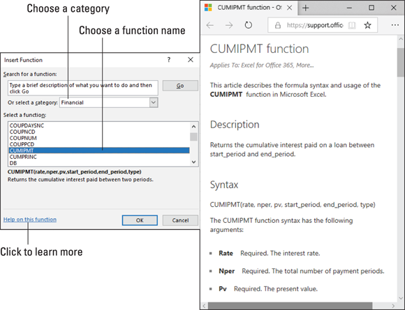
FIGURE 3-12: The Insert Function dialog box.
Using arguments in functions
Every function takes one or more arguments. Arguments are the cell references or numbers, enclosed in parentheses, that the function acts upon. For example, =AVERAGE(B1:B4) returns the average of the numbers in the cell range B1 through B4; =PRODUCT(6.5,C4) returns the product of multiplying the number 6.5 by the number in cell C4. When a function requires more than one argument, enter a comma between the arguments (enter a comma without a space).
Entering a function in a formula
To enter a function in a formula, you can enter the function name by typing it in the Formula bar, or you can rely on Excel to enter it for you. Enter function names yourself if you're well acquainted with a function and comfortable using it.
No matter how you want to enter a function as part of a formula, start this way:
- Select the cell where you want to enter the formula.
In the Formula bar, type an equals sign (=).
Please, please, please be sure to start every formula by entering an equals sign (=). Without it, Excel thinks you’re entering text or a number in the cell.Start constructing your formula, and when you come to the place where you want to enter the function, type the function’s name or call upon Excel to help you enter the function and its arguments.
The upcoming section, “Manually entering a function” shows how to type in the function yourself; “Getting Excel’s help to enter a function” shows how to get Excel to do the work.
If you enter the function on your own, it’s up to you to type the arguments correctly; if you get Excel’s help, you also get help with entering the cell references for the arguments.
Manually entering a function
Be sure to enclose the function’s argument or arguments in parentheses. Don’t enter a space between the function’s name and the first parenthesis. Likewise, don’t enter a comma and a space between arguments; enter a comma, nothing more:
=SUM(F11,F14,23)
You can enter function names in lowercase. Excel converts function names to uppercase after you click the Enter button or press Enter to complete the formula. Entering function names in lowercase is recommended because doing so gives you a chance to find out whether you entered a function name correctly. If Excel doesn’t convert your function name to uppercase, you made a typing error when you entered the function name.
Getting Excel’s help to enter a function
Besides entering a function by typing it, you can do it by way of the Function Arguments dialog box, as shown in Figure 3-13. The beauty of using this dialog box is that it warns you if you enter arguments incorrectly. What’s more, the Function Arguments dialog box shows you the results of the formula as you construct it so that you can tell whether you’re using the function correctly.
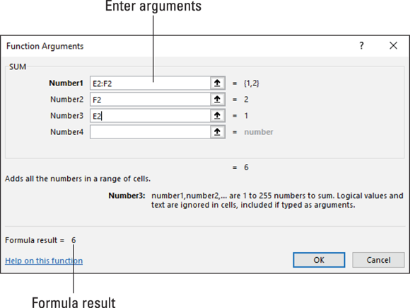
FIGURE 3-13: The Function Arguments dialog box.
Follow these steps to get Excel’s help with entering a function as part of a formula:
On the Formulas tab, tell Excel which function you want to use.
You can do that with one of these techniques:
- Click a Function Library button. Click the button whose name describes what kind of function you want and choose the function’s name on the drop-down list. You can click the Financial, Logical, Text, Date & Time, Lookup & Reference, Math & Trig, or More Functions buttons.
- Click the Recently Used button. Click this button and choose the name of a function you used recently.
- Click the Insert Function button. Clicking this button opens the Insert Function dialog box (refer to Figure 3-12). Find and choose the name of a function. You can search for functions or choose a category and then scroll the names until you find the function you want.
You see the Function Arguments dialog box (refer to Figure 3-13). It offers boxes for entering arguments for the function to compute.
Enter arguments in the spaces provided by the Function Arguments dialog box.
To enter cell references or ranges, you can click or select cells in your worksheet. If necessary, click the Range Selector button (you can find it to the right of an argument text box) to shrink the Function Arguments dialog box and get a better look at your worksheet.
Click OK when you finish entering arguments for your function.
I hope you didn’t have to argue too strenuously with the Function Arguments dialog box.
A Look at Some Very Useful Functions
Starting with Table 3-3, the remainder of this chapter looks into functions that I consider especially useful or interesting. After you spend some time constructing formulas, you’ll come up with your own list of useful or interesting functions.
TABLE 3-3 Common Functions and Their Use
Function |
Returns |
AVERAGE(number1,number2,…) |
The average of the numbers in the cells listed in the arguments |
COUNT(value1,value2,…) |
The number of cells that contain the numbers listed in the arguments |
MAX(number1,number2,…) |
The largest value in the cells listed in the arguments |
MIN(number1,number2,…) |
The smallest value in the cells listed in the arguments |
PRODUCT(number1,number2,…) |
The product of multiplying the cells listed in the arguments |
STDEV(number1,number2,…) |
An estimate of standard deviation based on the sample cells listed in the argument |
STDEVP(number1,number2,…) |
An estimate of standard deviation based on the entire sample cells listed in the arguments |
SUM(number1,number2,…) |
The total of the numbers in the arguments |
VAR(number1,number2,…) |
An estimate of the variance based on the sample cells listed in the arguments |
VARP(number1,number2,…) |
A variance calculation based on all cells listed in the arguments |
AVERAGE for averaging data
Might as well start with an easy one. The AVERAGE function averages the values in a cell range. In Figure 3-14, for example, AVERAGE is used to compute the average rainfall in a three-month period in three different counties.

FIGURE 3-14: Using AVERAGE to find average rainfall data.
Use AVERAGE as follows:
AVERAGE(cell range)
Excel ignores empty cells and logical values in the cell range; cells with 0 are computed.
COUNT and COUNTIF for tabulating data items
Use COUNT, a statistical function, to count how many cells have data in them. Numbers and dates, not text entries, are counted. The COUNT function is useful for tabulating how many data items are in a range. In the spreadsheet at the top of Figure 3-15, for example, COUNT is used to compute the number of mountains listed in the data:
COUNT(C5:C9)
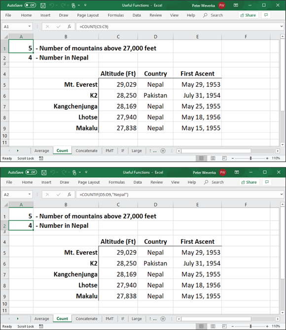
FIGURE 3-15: The COUNT (above) and COUNTIF (below) function at work.
Use COUNT as follows:
COUNT(cell range)
Similar to COUNT is the COUNTIF function. It counts how many cells in a cell range have a specific value. To use COUNTIF, enter the cell range and a criterion in the argument, as follows. If the criterion is a text value, enclose it in quotation marks.
COUNTIF(cell range, criterion)
At the bottom of Figure 3-15, the formula determines how many of the mountains in the data are in Nepal:
=COUNTIF(D5:D9,"Nepal")
CONCATENATE for combining values
CONCATENATE, a text function, is useful for combining values from different cells into a single cell. In the spreadsheet at the top of Figure 3-16, for example, values from three columns are combined in a fourth column to list peoples’ names in their entirety.
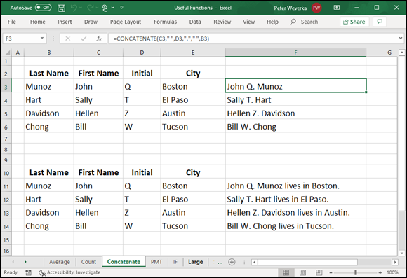
FIGURE 3-16: Use the CONCATENATE function to combine values from cells.
Use CONCATENATE as follows:
CONCATENATE(text1,text2,text3…)
To include blank spaces in the text you’re combining, enclose a blank space between quotation marks as an argument. Moreover, you can include original text in the concatenation formula as long as you enclose it in quotation marks and enter it as a separate argument. In Figure 3-16, I had to include a period after the middle initial, so in the formula, I entered a period in quotation marks as an argument:
=CONCATENATE(C3," ",D3,"."," ",B3)
In the spreadsheet shown at the bottom of Figure 3-16, I used the CONCATENATE function to write sentences (“John Q. Munoz lives in Boston.”). I included the words “lives in” in the formula, as follows:
=CONCATENATE(C11," ",D11,"."," ",B11," ","lives in"," ",E11,".")
PMT for calculating how much you can borrow
If you’re looking to buy a house, a car, or another expensive item for which you have to borrow money, the question to ask yourself is: How much can I borrow and make the monthly payment on the loan without stressing my budget unnecessarily? Can you safely make a monthly payment of $1,000, $1,500, $2,000? How much you can afford to pay each month to service a loan determines how much you can realistically borrow.
Use the PMT (payment) function to explore how much you can borrow given different interest rates and different amounts. PMT determines how much you have to pay annually on different loans. After you determine how much you have to pay annually, you can divide this amount by 12 to see how much you have to pay monthly.
Use the PMT function as follows to determine how much you pay annually for a loan:
PMT(interest rate, number of payments, amount of loan)
As shown in Figure 3-17, set up a worksheet with five columns to explore loan scenarios:
- Interest rate (column A): Because the interest rate on loans is expressed as a percentage, format this column to accept numbers as percentages (click the Percent Style button on the Home tab).
- No. of payments (column B): Typically, loan payments are made monthly. For a 30-year home loan mortgage, enter 360 in this column (12 months × 30 years); for a 15-year mortgage, enter 180 (12 months × 15 years). Enter the total number of loan payments you will make during the life of the loan.
- Amount of loan (column C): Enter the amount of the loan.
- Annual payment (column D): Enter a formula with the PMT function in this column to determine how much you have to pay annually for the loan. In Figure 3-17, the formula is
=PMT(A3,B3,C3) - Monthly payment (column E): Divide the annual payment in column D by 12 to determine the monthly payment:
=D3/12

FIGURE 3-17: Exploring loan scenarios with the PMT function.
After you set up the worksheet, you can start playing with different loan scenarios — different interest rates and amounts — to find out how much you can comfortably borrow and comfortably pay each month to pay back the loan.
IF for identifying data
The IF function examines data and returns a value based on criteria you enter. Use the IF function to locate data that meets a certain threshold. In the worksheet shown in Figure 3-18, for example, the IF function is used to identify teams that are eligible for the playoffs. To be eligible, a team must have won more than six games. The IF function identifies whether a team has won more than six games and, in the Playoffs column, enters the word Yes or No accordingly.

FIGURE 3-18: Exploring data with the IF function.
Use the IF function as follows:
IF(logical true-false test, value if true, value if false)
Instructing Excel to enter a value if the logical true-false test comes up false is optional; you must supply a value to enter if the test is true. Enclose the value in quotation marks if it is a text value such as the word Yes or No.
In Figure 3-18, the formula for determining whether a team made the playoffs is as follows:
=IF(C3>6,"Yes","No")
If the false “No” value was absent from the formula, teams that didn’t make the playoffs would not show a value in the Playoffs column; these teams’ Playoffs column would be empty.
LEFT, MID, and RIGHT for cleaning up data
Sometimes when you import data from another software application, especially if it’s a database application, the data arrives with unneeded characters. You can use the LEFT, MID, RIGHT, and TRIM functions to remove these characters:
- LEFT returns the leftmost characters in a cell to the number of characters you specify. For example, in a cell with CA_State, this formula returns CA, the two leftmost characters in the text:
=LEFT(A1,2) - MID returns the middle characters in a cell starting at a position you specify to the number of characters you specify. For example, in a cell with
http://www.dummies.com, this formula uses MID to remove the extraneous seven characters at the beginning of the URL and getwww.dummies.com:=MID(A1,7,50) - RIGHT returns the rightmost characters in a cell to the number of characters you specify. For example, in a cell containing the words Vitamin B1, this formula returns B1, the two rightmost characters in the name of the vitamin:
=RIGHT(A1,2) - TRIM, except for single spaces between words, removes all blank spaces from inside a cell. Use TRIM to remove leading and trailing spaces. This formula removes unwanted spaces from the data in cell A1:
=TRIM(A1)
PROPER for capitalizing words
The PROPER function makes the first letter of each word in a cell uppercase. As are LEFT and RIGHT, it is useful for cleaning up data you imported from elsewhere. Use PROPER as follows:
PROPER(cell address)
LARGE and SMALL for comparing values
Use the LARGE and SMALL functions, as well as their cousins MIN, MAX, and RANK, to find out where a value stands in a list of values. For example, use LARGE to locate the ninth oldest man in a list, or MAX to find the oldest man. Use MIN to find the smallest city by population in a list, or SMALL to find the fourth smallest. The RANK function finds the rank of a value in a list of values.
Use these functions as follows:
- MIN returns the smallest value in a list of values. For the argument, enter a cell range or cell array. In the worksheet shown in Figure 3-19, the following formula finds the fewest number of fish caught at any lake on any day:
=MIN(C3:G7) - SMALL returns the nth smallest value in a list of values. This function takes two arguments: first, the cell range or cell array, and next, the position, expressed as a number, from the smallest of all values in the range or array. In the worksheet shown in Figure 3-19, this formula finds the second smallest number of fish caught in any lake:
=SMALL(C3:G7,2) - MAX returns the largest value in a list of values. Enter a cell range or cell array as the argument. In the worksheet shown in Figure 3-19, this formula finds the most number of fish caught in any lake:
=MAX(C3:G7) - LARGE returns the nth largest value in a list of values. This function takes two arguments: first, the cell range or cell array, and next, the position, expressed as a number, from the largest of all values in the range or array. In the worksheet shown in Figure 3-19, this formula finds the second largest number of fish caught in any lake:
=LARGE(C3:G7,2) RANK returns the rank of a value in a list of values. This function takes three arguments:
- The cell with the value used for ranking
- The cell range or cell array with the comparison values for determining rank
- Whether to rank in order from top to bottom (enter 0 for descending) or bottom to top (enter 1 for ascending)
In the worksheet shown in Figure 3-19, this formula ranks the total number of fish caught in Lake Temescal against the total number of fish caught in all five lakes:
=RANK(H3,H3:H7,0)
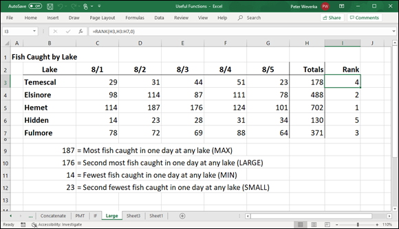
FIGURE 3-19: Using functions to compare values.
NETWORKDAY and TODAY for measuring time in days
Excel offers a couple of date functions for scheduling, project planning, and measuring time periods in days.
NETWORKDAYS measures the number of workdays between two dates (the function excludes Saturdays and Sundays from its calculations). Use this function for scheduling purposes to determine the number of workdays needed to complete a project. Use NETWORKDAYS as follows:
NETWORKDAYS(start date, end date)
TODAY gives you today’s date, whatever it happens to be. Use this function to compute today’s date in a formula. The TODAY function takes no arguments and is entered like so, parentheses included:
TODAY()
To measure the number of days between two dates, use the minus operator and subtract the latest date from the earlier one. For example, this formula measures the number of days between 1/1/2019 and 6/1/2019:
="6/1/2019"-"1/1/2019"
The dates are enclosed in quotation marks to make Excel recognize them as dates. Make sure that the cell where the formula is located is formatted to show numbers, not dates.
LEN for Counting Characters in Cells
Use the LEN (length) function to obtain the number of characters in a cell. This function is useful for making sure that characters remain under a certain limit. The LEN function counts blank spaces as well as characters. Use the LEN function as follows:
LEN(cell address)