Chapter 1
Up and Running with Excel
IN THIS CHAPTER
 Creating an Excel workbook
Entering text as well as numeric, date, and time data
Using the AutoFill command to enter lists and serial data
Setting up data-validation rules
This chapter introduces Microsoft Excel, the official number cruncher of Office 365. The purpose of Excel is to track, analyze, and tabulate numbers. Use the program to project profits and losses, formulate a budget, or analyze Elvis sightings in North America. Doing the setup work takes time, but after you enter the numbers and tell Excel how to tabulate them, you’re on Easy Street. Excel does the math for you. All you have to do is kick off your shoes, sit back, and see how the numbers stack up.
This chapter explains what a workbook and a worksheet is, and how rows and columns on a worksheet determine where cell addresses are. You also discover tips and tricks for entering data quickly in a worksheet and how to construct data-validation rules to make sure that data is entered accurately.
Creating a New Excel Workbook
Workbook is the Excel term for the files you create with Excel. When you create a workbook, you are given the choice of creating a blank workbook or creating a workbook from a template.
A template is a preformatted workbook designed for a specific purpose, such as budgeting, tracking inventories, or tracking purchase orders. Creating a workbook from a template is mighty convenient if you happen to find a template that suits your purposes, but in my experience, you almost always have to start from a generic, blank workbook because your data is your own. You need a workbook that you create yourself, not one created from a template by someone else.
To create a workbook, begin by going to the File tab and choosing New. You see the New window, shown in Figure 1-1. This window offers templates for creating workbooks and the means to search for templates online.
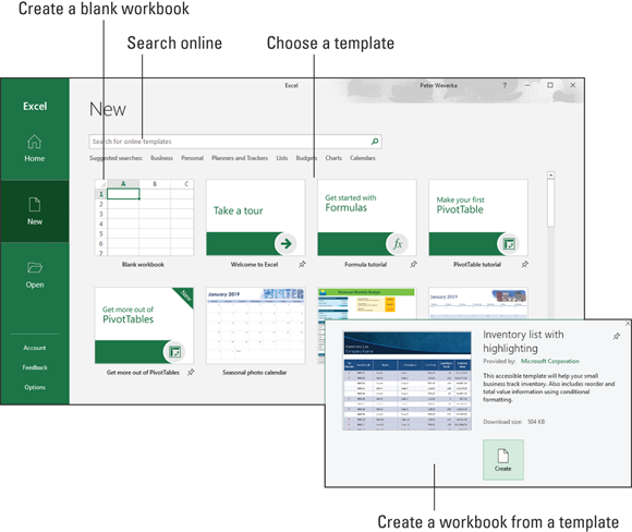
FIGURE 1-1: Create a workbook by starting in the New window.
Use these techniques in the New window to choose a template and create a workbook:
Choose the blank workbook template. Choose Blank Workbook to create a plain template.
 Press Ctrl+N to create a new, blank workbook without opening the New window.
- Choose a template. Select a template to examine it in a preview window (refer to Figure 1-1). If you like what you see, click the Create button in the preview window to create a document from the template.
- Search online for a template. Enter a search term in the Search box and click the Start Searching button (or click a suggested search term). New templates appear in the New window. Click a template to preview it (see Figure 1-1). Click the Create button in the preview window to create a document from the template.
Book 1, Chapter 1 explains how to save files after you create them, as well as how to open a file, including an Excel workbook.
Getting Acquainted with Excel
If you’ve spent any time in an Office application, much of the Excel screen may look familiar to you. The buttons on the Home tab — the Bold and the Align buttons, for example — work the same in Excel as they do in Word. The Font and Font Size drop-down lists work the same as well. Any command in Excel that has to do with formatting text and numbers works the same in Excel and Word.
As mentioned earlier, an Excel file is a workbook. Each workbook comprises one or more worksheets. A worksheet, also known as a spreadsheet, is a table into which you enter data and data labels. Figure 1-2 shows a worksheet with data about rainfall in different counties.

FIGURE 1-2: The Excel screen.
A worksheet works like an accountant’s ledger — only it’s much easier to use. Notice how the worksheet is divided by gridlines into columns (A, B, C, and so on) and rows (1, 2, 3, and so on). The rectangles where columns and rows intersect are cells, and each cell can hold one data item, a formula for calculating data, or nothing at all.
Each cell has a different cell address. In Figure 1-2, cell B7 holds 13, the number of inches of rain that fell in Sonoma County in the winter. Meanwhile, as the Formula bar at the top of the screen shows, cell F7, the active cell, holds the formula =B7+C7+D7+E7, the sum of the numbers in cells — you guessed it — B7, C7, D7, and E7.
 The beauty of Excel is that the program does all the calculations and recalculations for you after you enter the data. If I were to change the number in cell B7, Excel would instantly recalculate the total amount of rainfall in Sonoma County in cell F7. People like myself who struggled in math class will be glad to know that you don't have to worry about the math because Excel does it for you. All you have to do is make sure that the data and the formulas are entered correctly.
After you enter and label the data, enter the formulas, and turn your worksheet into a little masterpiece, you can start analyzing the data. For example, you can generate charts like the one in Figure 1-3. Do you notice any similarities between the worksheet in Figure 1-2 and the chart in Figure 1-3? The chart is fashioned from data in the worksheet, and it took me about half a minute to create that chart. (Book 8, Chapter 1 explains how to create charts in Excel, Word, and PowerPoint.)
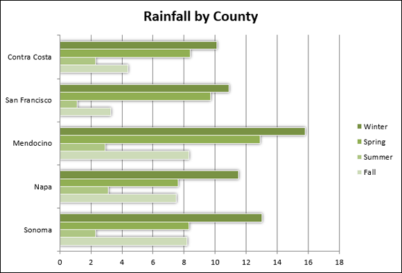
FIGURE 1-3: A chart generated from the data in Figure 1-2.
Rows, columns, and cell addresses
Not that anyone needs them all, but an Excel worksheet has numerous columns and more than 1 million rows. The rows are numbered, and columns are labeled A to Z, then AA to AZ, then BA to BZ, and so on. The important thing to remember is that each cell has an address whose name comes from a column letter and a row number. The first cell in row 1 is A1, the second is B1, and so on. You need to enter cell addresses in formulas to tell Excel which numbers to compute.
To find a cell's address, either make note of which column and row it lies in or click the cell and glance at the Formula bar (refer to Figure 1-2). The left side of the Formula bar lists the address of the active cell, the cell that is selected in the worksheet. In Figure 1-2, cell F7 is the active cell.
Workbooks and worksheets
By default, each workbook includes one worksheet, called Sheet1, but you can add more worksheets (and rename worksheets, too). Think of a workbook as a stack of worksheets. Besides calculating the numbers in cells across the rows or down the columns of a worksheet, you can make calculations throughout a workbook by using numbers from different worksheets in a calculation. Chapter 2 of this minibook explains how to add worksheets, rename worksheets, and do all else that pertains to them.
Entering Data in a Worksheet
Entering data in a worksheet is an irksome activity. Fortunately, Excel offers a few shortcuts to take the sting out of it. These pages explain how to enter data in a worksheet, what the different types of data are, and how to enter text labels, numbers, dates, and times.
The basics of entering data
What you can enter in a worksheet cell falls into four categories:
- Text
- A value (numeric, date, or time)
- A logical value (True or False)
- A formula that returns a value, logical value, or text
Still, no matter what type of data you're entering, the basic steps are the same:
Click the cell where you want to enter the data or text label.
As shown in Figure 1-4, a square appears around the cell to tell you that the cell you clicked is now the active cell. Glance at the left side of the Formula bar if you're not sure of the address of the cell you’re about to enter data in. The Formula bar lists the cell address.
Type the data in the cell.
If you find typing in the Formula bar easier, click and start typing there.
Press the Enter key to enter the number or label.
Besides pressing the Enter key, you can also press an arrow key (←, ↑, →, ↓), press Tab, click the Enter button (the check mark) on the Formula bar, or click elsewhere on the worksheet.
If you change your mind about entering data, click the Cancel button or press Esc to delete what you entered and start over. The Cancel button (an X) is located on the Formula bar next to the Enter button (a check mark) and the Insert Function button (labeled fx).

FIGURE 1-4: Entering data.
Chapter 3 of this minibook explains how to enter logical values and formulas. The next several pages describe how to enter text labels, numeric values, date values, and time values.
Entering text labels
Sometimes a text entry is too long to fit in a cell. How Excel accommodates text entries that are too wide depends on whether data is in the cell to the right of the one you entered the text in:
- If the cell to the right is empty, Excel lets the text spill into the next cell.
- If the cell to the right contains data, the entry gets cut off. Nevertheless, the text you entered is in the cell. Nothing gets lost when it can't be displayed onscreen. You just can’t see the text or numbers except by glancing at the Formula bar, where the contents of the active cell can be seen in their entirety.
Use these techniques to solve the problem of text that doesn’t fit in a cell:
- Widen the column to allow room for more text.
- Shorten the text entry.
- Reorient the text (Chapter 4 of this minibook explains how to do it).
- Wrap the contents of the cell. Wrapping means to run the text down to the next line, much the same way as the text in a paragraph runs to the next line when it reaches the right margin. Excel makes rows taller to accommodate wrapped text in a cell. To wrap text in cells, select the cells, go to the Home tab, and click the Wrap Text button (found in the Alignment group).
Entering numeric values
When a number is too large to fit in a cell, Excel displays pounds signs (###) instead of a number or displays the number in scientific notation (8.78979E+15). You can always glance at the Formula bar, however, to find out the number in the active cell. As well, you can always widen the column to display the entire number.
To enter a fraction in a cell, enter a 0 or a whole number, a blank space, and the fraction. For example, to enter 3⁄8, type a 0, press the spacebar, and type 3/8. To enter 53⁄8, type 5, press the spacebar, and type 3/8. For its purposes, Excel converts fractions to decimal numbers, as you can see by looking in the Formula bar after you enter a fraction. For example, 53⁄8 displays as 5.375 in the Formula bar.
Here’s a little trick for entering numbers with decimals quickly in all the Excel files you work on. To spare yourself the trouble of pressing the period key (.), you can tell Excel to enter the period automatically. Instead of entering 12.45, for example, you can simply enter 1245. Excel enters the period for you: 12.45. To perform this trick, go to the File tab, choose Options, visit the Advanced category in the Excel Options dialog box, click the Automatically Insert a Decimal Point check box, and in the Places text box, enter the number of decimal places you want for numbers. Deselect this option when you want to go back to entering numbers the normal way.
Entering date and time values
Dates and times can be used in calculations, but entering a date or time value in a cell can be problematic because these values must be entered in such a way that Excel can recognize them as dates or times, not text.
 Not that you necessarily need to know it, but Excel converts dates and times to serial values for the purpose of being able to use dates and times in calculations. For example, July 31, 2004, is the number 38199. July 31, 2004, at noon is 38199.5. These serial values represent the number of whole days since January 1, 1900. The portion of the serial value to the right of the decimal point is the time, represented as a portion of a full day.
Entering date values
You can enter a date value in a cell in just about any format you choose, and Excel understands that you’re entering a date. For example, enter a date in any of the following formats and you’ll be all right:
m/d/yy |
7/31/19 |
m-d-yyyy |
7-31-2019 |
d-mmm-yy |
31-Jul-19 |
Here are some basic things to remember about entering dates:
- Date formats: You can quickly apply a format to dates by selecting cells and using one of these techniques:
- On the Home tab, open the Number Format drop-down list and choose Short Date (m/d/yyyy; 7/31/2016) or Long Date (day of the week, month, day, year; Wednesday, July 31, 2016), as shown in Figure 1-5.
- On the Home tab, click the Number group button to open the Number tab of the Format Cells dialog box. As shown in Figure 1-5, choose the Date category and then choose a date format.
- Current date: Press Ctrl+; (semicolon) to enter the current date.
- Current year’s date: If you don’t enter the year as part of the date, Excel assumes that the date you entered is in the current year. For example, if you enter a date in the m/d (7/31) format during the year 2019, Excel enters the date as 7/31/19. As long as the date you want to enter is the current year, you can save a little time when entering dates by not entering the year because Excel enters it for you.
- Dates on the Formula bar: No matter which format you use for dates, dates are displayed in the Formula bar in the format that Excel prefers for dates: m/d/yyyy (7/31/2019). How dates are displayed in the worksheet is up to you.
- Twentieth and twenty-first century two-digit years: When it comes to entering two-digit years in dates, the digits 30 through 99 belong to the twentieth century (1930–1999), but the digits 00 through 29 belong to the twenty-first century (2000–2029). For example, 7/31/13 refers to July 31, 2013, not July 31, 1910. To enter a date in 1929 or earlier, enter four digits instead of two to describe the year: 7-31-1929. To enter a date in 2030 or later, enter four digits instead of two: 7-31-2030.
- Dates in formulas: To enter a date directly in a formula, enclose the date in quotation marks. (Make sure that the cell where the formula is entered has been given the Number format, not the Date format.) For example, the formula
=TODAY()-“1/1/2019”calculates the number of days that have elapsed since January 1, 2019. Formulas are the subject of Chapter 3 of this minibook.

FIGURE 1-5: Format dates and numbers on the Number Format drop-down list or Format Cells dialog box.
Entering time values
Excel recognizes time values that you enter in the following ways:
h:mm AM/PM |
3:31 AM |
h:mm:ss AM/PM |
3:31:45 PM |
Here are some things to remember when entering time values:
- Use colons: Separate hours, minutes, and seconds with a colon (:).
- Time formats: To change to the h:mm:ss AM/PM time format, select the cells, go to the Home tab, open the Number Format drop-down list, and choose Time (see Figure 1-5). You can also change time formats by clicking the Number group button on the Home tab and selecting a time format on the Number tab of the Format Cells dialog box.
- AM or PM time designations: Unless you enter AM or PM with the time, Excel assumes that you’re operating on military time. For example, 3:30 is considered 3:30 a.m.; 15:30 is 3:30 p.m. Don’t enter periods after the letters am or pm (don’t enter a.m. or p.m.).
- Current time: Press Ctrl+Shift+; (semicolon) to enter the current time.
- Times on the Formula bar: On the Formula bar, times are displayed in this format: hours:minutes:seconds, followed by the letters AM or PM. However, the time format used in cells is up to you.
Combining date and time values
You can combine dates and time values by entering the date, a blank space, and the time:
- 7/31/13 3:31 am
- 7-31-13 3:31:45 pm
Quickly Entering Lists and Serial Data with the AutoFill Command
Data that falls into the “serial” category — month names, days of the week, and consecutive numbers and dates, for example — can be entered quickly with the AutoFill command. Believe it or not, Excel recognizes certain kinds of serial data and enters it for you as part of the AutoFill feature. Instead of laboriously entering this data one piece at a time, you can enter it all at one time by dragging the mouse. Follow these steps to “autofill” cells:
Click the cell that is to be first in the series.
For example, if you intend to list the days of the week in consecutive cells, click where the first day is to go.
- Enter the first number, date, or list item in the series.
Move to the adjacent cell and enter the second number, date, or list item in the series.
If you want to enter the same number or piece of text in adjacent cells, taking this step isn't necessary, but Excel needs the first and second items in the case of serial dates and numbers so that it can tell how much to increase or decrease the given amount or time period in each cell. For example, entering 5 and 10 tells Excel to increase the number by 5 each time so that the next serial entry is 15.
Select the cell or cells you just entered data in.
To select a single cell, click it; to select two, drag over the cells. Chapter 2 of this minibook describes all the ways to select cells in a worksheet.
Click the AutoFill handle and start dragging in the direction in which you want the data series to appear on your worksheet.
The AutoFill handle is the little green square in the lower-right corner of the cell or block of cells you selected. As you drag, the serial data appears in a pop-up box, as shown in Figure 1-6.

FIGURE 1-6: Entering serial data and text.
The AutoFill Options button appears after you enter the serial data. Click it and choose an option if you want to copy cells or fill the cells without carrying along their formats.
To enter the same number or text in several empty cells, drag over the cells to select them or select each cell by holding down the Ctrl key as you click. Then type a number or some text and press Ctrl+Enter.
Formatting Numbers, Dates, and Time Values
When you enter a number that Excel recognizes as belonging to one of its formats, Excel assigns the number format automatically. Enter 45%, for example, and Excel assigns the Percentage number format. Enter $4.25, and Excel assigns the Currency number format. Besides assigning formats by hand, however, you can assign them to cells from the get-go and spare yourself the trouble of entering dollar signs, commas, percent signs, and other extraneous punctuation. All you have to do is enter the raw numbers. Excel does the window dressing for you.
Excel offers five number-formatting buttons on the Home tab. Select cells with numbers in them and click one of these buttons to change how numbers are formatted:
- Accounting Number Format: Places a dollar sign before the number and gives it two decimal places. You can open the drop-down list on this button and choose a currency symbol apart from the dollar sign.
- Percent Style: Places a percent sign after the number and converts the number to a percentage.
- Comma Style: Places commas in the number.
- Increase Decimal: Increases the number of decimal places by one.
- Decrease Decimal: Decreases the number of decimal places by one.
To choose among many formats and to format dates and time values as well as numbers, go to the Home tab, click the Number group button, and make selections on the Number tab of the Format Cells dialog box. Figure 1-7 shows this dialog box. Choose a category and select options to describe how you want numbers or text to appear.
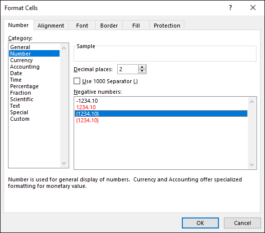
FIGURE 1-7: The Number category of the Format Cells dialog box.
To strip formats from the data in cells, select the cells, go to the Home tab, click the Clear button, and choose Clear Formats.
Entering ZIP codes can be problematic because Excel strips the initial zero from the number if it begins with a zero. To get around this problem, visit the Number tab of the Format Cells dialog box (see Figure 1-7), choose Special in the Category list, and select a ZIP code option.
Establishing Data-Validation Rules
By nature, people are prone to enter data incorrectly because the task of entering data is so dull. This is why data-validation rules are invaluable. A data-validation rule is a rule concerning what kind of data can be entered in a cell. When you select a cell that has been given a rule, an input message tells you what to enter, as shown in Figure 1-8. And if you enter the data incorrectly, an error alert tells you as much, also shown in Figure 1-8.
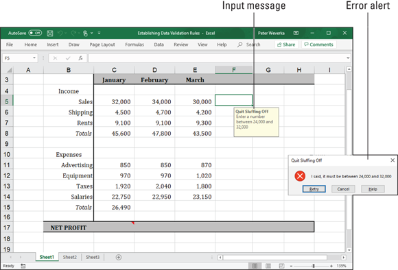
FIGURE 1-8: A data-validation rule in action.
Data-validation rules are an excellent defense against sloppy data entry and that itchy feeling you get when you’re in the middle of an irksome task. In a cell that records date entries, you can require dates to fall in a certain time frame. In a cell that records text entries, you can choose an item from a list instead of typing it yourself. In a cell that records numeric entries, you can require the number to fall within a certain range. Table 1-1 describes the different categories of data-validation rules.
TABLE 1-1 Data-Validation Rule Categories
Rule |
What Can Be Entered |
Any Value |
Anything whatsoever. This is the default setting. |
Whole Number |
Whole numbers (no decimal points allowed). Choose an operator from the Data drop-down list and values to describe the range of numbers that can be entered. |
Decimal |
Same as the Whole Number rule except numbers with decimal points are permitted. |
List |
Items from a list. Enter the list items in cells on a worksheet, either the one you’re working in or another. Then reopen the Data Validation dialog box, click the Range Selector button (you can find it on the right side of the Source text box), and select the cells that hold the list. The list items appear in a drop-down list on the worksheet. |
Date |
Date values. Choose an operator from the Data drop-down list and values to describe the date range. Earlier in this chapter, “Entering date and time values” describes the correct way to enter date values. |
Time |
Time values. Choose an operator from the Data drop-down list and values to describe the date and time range. Earlier in this chapter, “Entering date and time values” describes the correct way to enter a combination of date and time values. |
Text Length |
A certain number of characters. Choose an operator from the Data drop-down list and values to describe how many characters can be entered. |
Custom |
A logical value (True or False). Enter a formula that describes what constitutes a true or false data entry. |
Follow these steps to establish a data-validation rule:
- Select the cell or cells that need a rule.
On the Data tab, click the Data Validation button.
As shown in Figure 1-9, you see the Settings tab of the Data Validation dialog box.
On the Allow drop-down list, choose the category of rule you want.
Table 1-1, earlier in this chapter, describes these categories.
Enter the criteria for the rule.
What the criteria is depends on what rule category you’re working in. Table 1-1 describes how to enter the criteria for rules in each category. You can refer to cells in the worksheet by selecting them. To do that, either select them directly or click the Range Selector button and then select them.
On the Input Message tab, enter a title and input message.
You can see a title (“Quit Sluffing Off”) and input message (“Enter a number between 24,000 and 32,000”) in Figure 1-8. The title appears in boldface. Briefly describe what kind of data belongs in the cell or cells you selected.
On the Error Alert tab, choose a style for the symbol in the Message Alert dialog box, enter a title for the dialog box, and enter a warning message.
In the error message in Figure 1-8, shown previously, the Stop symbol was chosen. The title you enter appears across the top of the dialog box, and the message appears beside the symbol.
Click OK.
To remove data-validation rules from cells, select the cells, go to the Data tab, click the Data Validation button, and on the Settings tab of the Data Validation dialog box, click the Clear All button, and click OK.
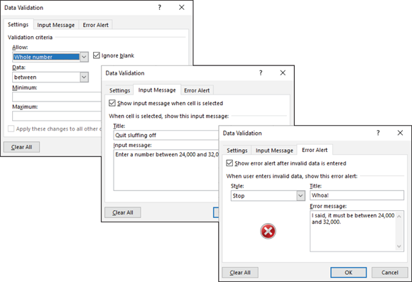
FIGURE 1-9: Creating a data-validation rule.