Chapter 5

Advanced Techniques for Analyzing Data

IN THIS CHAPTER

Using conditional formats to call attention to data

Sorting and filtering information in a worksheet list

Performing what-if analyses with data tables

Examining data with a PivotTable

This chapter offers a handful of tricks for analyzing the data that you so carefully and lovingly enter in a worksheet. Delve into this chapter to find out what sparklines are and how to manage, sort, and filter data in lists. You also discover how conditional formats can help data stand out, how the Goal Seek command can help you target values in different kinds of analyses, and how you can map out different scenarios with data by using one- and two-input data tables. Finally, this chapter explains how a PivotTable can help turn an indiscriminate list into a meaningful source of information.

Seeing What the Sparklines Say

Maybe the easiest way to analyze information in a worksheet is to see what the sparklines say. Figure 5-1 shows examples of sparklines. In the form of a tiny line or bar chart, sparklines tell you about the data in a row or column.

FIGURE 5-1: Sparklines in action (top to bottom): Column, Line, and Win/Loss.

Follow these steps to create a sparkline chart:

1. Select the cell where you want the chart to appear.

2. On the Insert tab, click the Line, Column, or Win/Loss button.

   The Create Sparklines dialog box appears.

3. Drag in a row or column of your worksheet to select the cells with the data you want to analyze.
4. Click OK in the Create Sparklines dialog box.

To change the look of a sparkline chart, go to the (Sparkline Tools) Design tab. There you will find commands for changing the color of the line or bars, choosing a different sparkline type, and doing one or two other things to pass the time on a rainy day. Click the Clear button to remove a sparkline chart.

You can also create a sparkline chart with the Quick Analysis button. Drag over the cells with the data you want to analyze. When the Quick Analysis button appears, click it, choose Sparklines in the pop-up window, and then choose Line, Column, or Win/Loss.

Conditional Formats for Calling Attention to Data

A conditional format is one that applies when data meets certain conditions. To call attention to numbers greater than 10,000, for example, you can tell Excel to highlight those numbers automatically. To highlight negative numbers, you can tell Excel to display them in bright red. Conditional formats help you analyze and understand data better.

Select the cells that are candidates for conditional formatting and follow these steps to tell Excel when and how to format the cells:

1. On the Home tab, click the Conditional Formatting button (you may have to click the Styles button first, depending on the size of your screen).

2. Choose Highlight Cells Rules or Top/Bottom Rules on the drop-down list.

   You see a submenu with choices about establishing the rule for whether values in the cells are highlighted or otherwise made more prominent:

   • Highlight Cells Rules: These rules are for calling attention to data if it falls in a numerical or date range, or it’s greater or lesser than a specific value. For example, you can highlight cells that are greater than 400.
   • Top/Bottom Rules: These rules are for calling attention to data if it falls within a percentage range relative to all the cells you selected. For example, you can highlight cells with data that falls in the bottom 10-percent range.

3. Choose an option on the submenu.

   You see a dialog box similar to the ones in Figure 5-2.

4. On the left side of the dialog box, establish the rule for flagging data.

5. On the With drop-down list, choose how you want to call attention to the data.

   For example, you can display the data in red or yellow. You can choose Custom Format on the drop-down list to open the Format Cells dialog box and choose a font style or color for the text.

6. Click OK.

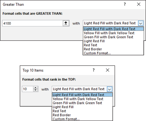
FIGURE 5-2: Establishing a condition format for data.

To remove conditional formats, select the cells with the formats, go to the Home tab, click the Conditional Formatting button, and choose Clear Rules⇒    Clear Rules from Selected Cells.

You can also establish conditional formats by selecting cells and pressing Ctrl+Q or clicking the Quick Analysis button (which appears next to cells after you select them). In the pop-up window, choose Formatting and then click Greater Than or Top 10% to create a highlight-cell or top/bottom rule.

Managing Information in Lists

Although Excel is a spreadsheet program, many people use it to keep and maintain lists, such as the list shown in Figure 5-3. Addresses, inventories, and employee data are examples of information that typically is kept in lists. These pages explain how to sort and filter a list to make it yield more information. Sort a list to put it in alphabetical or numeric order; filter a list to isolate the information you need.

FIGURE 5-3: A list in a worksheet.

Before you attempt a sort or filter operation, use the Format As Table command to capture the data you want to sort or filter in a list. Chapter 4 of this minibook explains how to format cells so that they form a table. (Hint: Select the cells, click the Format As Table button on the Home tab, and select a table style in the gallery.)

Sorting a list

Sorting means to rearrange the rows in a list on the basis of data in one or more columns. Sort a list on the Last Name column, for example, to arrange the list in alphabetical order by last name. Sort a list on the ZIP Code column to arrange the rows in numerical order by ZIP code. Sort a list on the Birthday column to arrange it chronologically from earliest born to latest born.

Here are all the ways to sort a list:

• Sorting on a single column: Click any cell in the column you want to use as the basis for the sort. For example, to sort item numbers from smallest to largest, click in the Item Number column. Then use one of these techniques to conduct the sort operation:
  • On the Data tab, click the Sort Smallest to Largest or Sort Largest to Smallest button. These buttons are located in the Sort & Filter group.
  • Open the drop-down menu on the column heading and choose Sort Smallest to Largest or Sort Largest to Smallest on the drop-down menu (see Figure 5-3). Click the Filter button on the Data tab if you don’t see the drop-down menus.
• Sorting on more than one column: Click the Sort button on the Data tab. You see the Sort dialog box, as shown in Figure 5-4. Choose which columns you want to sort with and the order in which you want to sort. To add a second or third column for sorting, click the Add Level button.

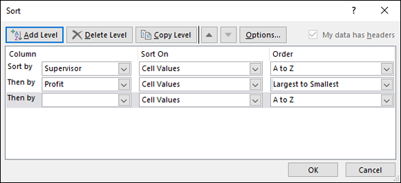
FIGURE 5-4: Sort to arrange the list data in different ways.

Filtering a list

Filtering means to scour a worksheet list for certain kinds of data. To filter, you tell Excel what kind of data you’re looking for, and the program assembles rows with that data to the exclusion of rows that don’t have the data. You end up with a shorter list with only the rows that match your filter criteria. Filtering is similar to using the Find command except that you get more than one row in the results of the filtering operation. For example, in a list of addresses, you can filter for addresses in California. In a price list, you can filter for items that fall within a certain price range.

To filter data, your list needs column headers, the descriptive labels in the first row that describe what is in the columns below. Excel needs column headers to identify and be able to filter the data in the rows. Each column header must have a different name.

To filter a list, start by going to the Data tab and clicking the Filter button. As shown in Figure 5-5, a drop-down list appears beside each column header.

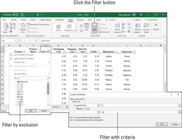
FIGURE 5-5: Filter a worksheet to isolate data.

Your next task is to open a drop-down list in the column that holds the criteria you want to use to filter the list. For example, if you want to filter the list to show items that cost more than $100, open the Cost column drop-down list; if you want to filter the list so that only the names of employees who make less than $30,000 annually appear, open the Salary drop-down list.

After you open the correct column drop-down list, tell Excel how you want to filter the list:

• Filter by exclusion: On the drop-down list, deselect the Select All check box and then select the check box next to each item you don’t want to filter out. For example, to filter an Address list for addresses in Boston, Chicago, and Miami, deselect the Select All check box and then select the check boxes next to Boston, Chicago, and Miami on the drop-down list. Your filter operation turns up only addresses in those three cities.

• Filter with criteria: On the drop-down list, choose Number Filters, and then choose a filter operation on the submenu (or simply choose Custom Filter). You see the Custom AutoFilter dialog box.

  Choose an operator (equals, is greater than, or another) from the drop-down list, and either enter or choose a target criterion from the list on the right side of the dialog box. You can search by more than one criterion. Select the And option button if a row must meet both criteria to be selected, or select the Or option button if a row can meet either criterion to be selected.

Click the OK button on the column’s drop-down list or the Custom AutoFilter dialog box to filter your list.

To see all the data in the list again — to unfilter the list — click the Clear button on the Data tab.

Forecasting with the Goal Seek Command

In a conventional formula, you provide the raw data, and Excel produces the results. With the Goal Seek command, you declare what you want the results to be, and Excel tells you the raw data that you need to produce those results. The Goal Seek command is useful in analyses when you want the outcome to be a certain way and you need to know which raw numbers will produce the outcome that you want.

Figure 5-6 shows a worksheet designed to find out the monthly payment on a mortgage. With the PMT function, the worksheet determines that the monthly payment on a $250,000 loan with an interest rate of 6.5 percent and to be paid over a 30-year period is $1,580.17. Suppose, however, that the person who calculated this monthly payment determined that he or she could pay more than $1,580.17 per month. Suppose that the person could pay $1,750 or $2,000 per month. Instead of an outcome of $1,580.17, the person wants to know how much he or she could borrow if monthly payments — the outcome of the formula — were increased to $1,750 or $2,000.

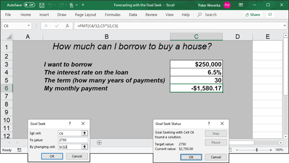
FIGURE 5-6: Experimenting with the Goal Seek command.

To make determinations such as these, you can use the Goal Seek command. This command lets you experiment with the arguments in a formula to achieve the results you want. In the case of the worksheet in Figure 5-6, you can use the Goal Seek command to change the argument in cell C3, the total amount you can borrow, given the outcome you want in cell C6, $1,750 or $2,000, the monthly payment on the total amount.

Follow these steps to use the Goal Seek command to change the inputs in a formula to achieve the results you want:

1. Select the cell with the formula whose arguments you want to experiment with.

2. On the Data tab, click the What-If Analysis button and choose Goal Seek on the drop-down list.

   You see the Goal Seek dialog box, shown in Figure 5-6. The address of the cell you selected in Step 1 appears in the Set Cell box.

3. In the To Value text box, enter the target results you want from the formula.

   In the example in Figure 5-6, you enter -1750 or -2000, the monthly payment you can afford for the 30-year mortgage.

4. In the By Changing Cell text box, enter the address of the cell whose value is unknown.

   To enter a cell address, go outside the Goal Seek dialog box and click a cell on your worksheet. In Figure 5-6, you select the address of the cell that shows the total amount you want to borrow.

5. Click OK.

   The Goal Seek Status dialog box appears, as shown in Figure 5-6. It lists the target value that you entered in Step 3.

6. Click OK.

   On your worksheet, the cell with the argument you wanted to alter now shows the target you’re seeking. In the case of the example worksheet in Figure 5-6, you can borrow $316,422 at 6.5 percent, not $250,000, by raising your monthly mortgage payments from $1,580.17 to $2,000.

Performing What-If Analyses with Data Tables

For something a little more sophisticated than the Goal Seek command (which I describe in the preceding section), try performing what-if analyses with data tables. With this technique, you change the data in input cells and observe what effect changing the data has on the results of a formula. The difference between the Goal Seek command and a data table is that with a data table, you can experiment simultaneously with many different input cells and in so doing experiment with many different scenarios.

Using a one-input table for analysis

In a one-input table, you find out what the different results of a formula would be if you changed one input cell in the formula. In Figure 5-7, that input cell is the interest rate on a loan. The purpose of this data table is to find out how monthly payments on a $250,000, 30-year mortgage are different, given different interest rates. The interest rate in cell B4 is the input cell.

FIGURE 5-7: A one-input data table.

Follow these steps to create a one-input table:

1. On your worksheet, enter values that you want to substitute for the value in the input cell.

   To make the input table work, you have to enter the substitute values in the right location:

   • In a column: Enter the values in the column starting one cell below and one cell to the left of the cell where the formula is located. In Figure 5-7, for example, the formula is in cell E4 and the values are in the cell range D5:D15.
   • In a row: Enter the values in the row starting one cell above and one cell to the right of the cell where the formula is.

2. Select the block of cells with the formula and substitute values.

   Select a rectangle of cells that encompasses the formula cell, the cell beside it, all the substitute values, and the empty cells where the new calculations will soon appear.

   • In a column: Select the formula cell, the cell to its left, all the substitute-value cells, and the cells below the formula cell.
   • In a row: Select the formula cell, the cell above it, the substitute values in the cells directly to the right, and the now-empty cells where the new calculations will appear.

3. On the Data tab, click the What-If Analysis button and choose Data Table on the drop-down list.

   You see the Data Table dialog box (refer to Figure 5-7).

4. In the Row Input Cell or Column Input Cell text box, enter the address of the cell where the input value is located.

   To enter this cell address, go outside the Data Table dialog box and click the cell. The input value is the value you’re experimenting with in your analysis. In the case of the worksheet shown in Figure 5-7, the input value is located in cell B4, the cell that holds the interest rate.

   If the new calculations appear in rows, enter the address of the input cell in the Row Input Cell text box; if the calculations appear in columns (refer to Figure 5-7), enter the input cell address in the Column Input Cell text box.

5. Click OK.

   Excel performs the calculations and fills in the table.

To generate the one-input table, Excel constructs an array formula with the TABLE function. If you change the cell references in the first row or plug in different values in the first column, Excel updates the one-input table automatically.

Using a two-input table for analysis

In a two-input table, you can experiment with two input cells rather than one. Getting back to the example of the loan payment in Figure 5-7, you can calculate not only how loan payments change as interest rates change but also how payments change if the life of the loan changes. Figure 5-8 shows a two-input table for examining monthly loan payments given different interest rates and two different terms for the loan: 15 years (180 months) and 30 years (360 months).

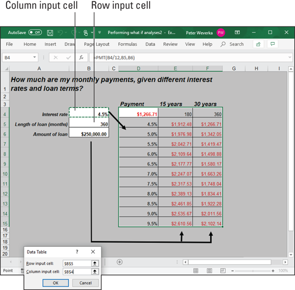
FIGURE 5-8: A two-input data table.

Follow these steps to create a two-input data table:

1. Enter one set of substitute values below the formula in the same column as the formula.

   In Figure 5-8, different interest rates are entered in the cell range D5:D15.

2. Enter the second set of substitute values in the row to the right of the formula.

   In Figure 5-8, 180 and 360 are entered. These numbers represent the number of months of the life of the loan.

3. Select the formula and all substitute values.

   Do this correctly and you select three columns, including the formula, the substitute values below it, and the two columns to the right of the formula. You select a big block of cells (the range D4:F15, in this example).

4. On the Data tab, click the What-If Analysis button and choose Data Table on the drop-down list.

   The Data Table dialog box appears (refer to Figure 5-8).

5. In the Row Input Cell text box, enter the address of the cell referred to in the original formula where substitute values to the right of the formula can be plugged in.

   Enter the cell address by going outside the dialog box and selecting a cell. In Figure 5-8, for example, the rows to the right of the formula are for length-of-loan substitute values. Therefore, I select cell B5, the cell referred to in the original formula where the length of the loan is listed.

6. In the Column Input Cell text box, enter the address of the cell referred to in the original formula where substitute values below the formula are.

   In Figure 5-8, the substitute values below the formula cell are interest rates. Therefore, I select cell B4, the cell referred to in the original formula where the interest rate is entered.

7. Click OK.

   Excel performs the calculations and fills in the table.

Analyzing Data with PivotTables

PivotTables give you the opportunity to reorganize data in a long worksheet list and in so doing analyze the data in new ways. You can display data such that you focus on one aspect of the list. You can turn the list inside out and perhaps discover things you didn’t know before.

When you create a PivotTable, what you really do is turn a multicolumn list into a table for the purpose of analysis. For example, the four-column list in Figure 5-9 records items purchased in two grocery stores over a four-week period. The four columns are

• Item: The items purchased
• Store: The grocery store (Safepath or Wholewallet) where the items were purchased
• Cost: The cost of the items
• Week: When the items were purchased (Week 1, 2, 3, or 4)

FIGURE 5-9: A raw multicolumn list (left) turned into meaningful PivotTables (right).

This raw list doesn’t reveal anything; it’s hardly more than a data dump. However, as Figure 5-9 shows, by turning the list into PivotTables, you can tease the list to find out, among other things:

• How much was spent item by item in each grocery store, with the total spent for each item (Sum of Cost by Item and Store)
• How much was spent on each item (Sum of Cost by Item)
• How much was spent at each grocery store (Sum of Cost by Store)
• How much was spent each week (Sum of Cost by Week)

Make sure that the list you want to analyze with a PivotTable has column headers. Column headers are the descriptive labels that appear across the top of columns in a list. Excel needs column headers to construct PivotTables.

Getting a PivotTable recommendation from Excel

The easiest way to create a PivotTable is to let Excel do the work. Follow these steps:

1. Select a cell anywhere in your data list.

2. On the Insert tab, click the Recommended PivotTables button.

   The Recommended PivotTables dialog box appears, as shown in Figure 5-10. This dialog box presents a number of PivotTables.

3. Scroll the list of PivotTables on the left side of the dialog box, selecting each one and examining it on the right side of the dialog box.

4. Select a PivotTable and click OK.

   The PivotTable appears on a new worksheet.

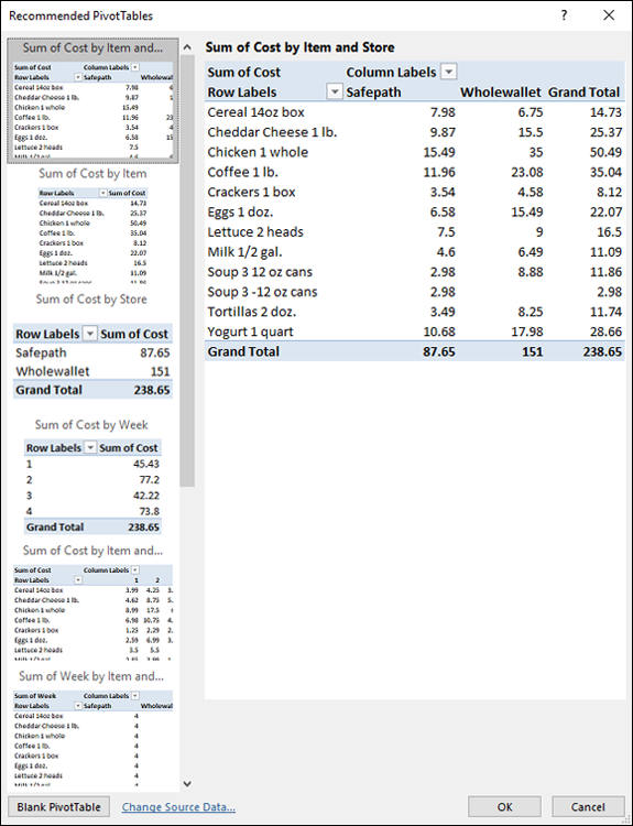
FIGURE 5-10: These PivotTables come highly recommended.

Creating a PivotTable from scratch

Follow these steps to create a PivotTable on your own:

1. Select a cell anywhere in your data list.

2. On the Insert tab, click the PivotTable button.

   Excel selects what it believes is your entire list, and you see the Create PivotTable dialog box. If the list isn’t correctly selected, click outside the dialog box and select the data you want to analyze.

3. Choose the New Worksheet option and click OK.

   You can choose the Existing Worksheet option and select cells on your worksheet to show Excel where you want to place the PivotTable, but in my experience, creating it on a new worksheet and moving it later is the easier way to go.

   The (PivotTable Tools) Analyze tab and PivotTable Fields task pane appear, as shown in Figure 5-11. The task pane lists the names of fields, or column headings, from your table.

4. In the PivotTable Fields task pane, drag field names into the four areas (Filters, Columns, Rows, and Values) to construct your PivotTable.

   As you construct your table, you see it take shape onscreen. You can drag fields in and out of areas as you please. Drag one field name into each of these areas:

   • Rows: The field whose data you want to analyze.
   • Columns: The field by which you want to measure and compare data.
   • Values: The field with the values used for comparison.
   • Filters (optional): A field you want to use to sort table data. (This field’s name appears in the upper-left corner of the PivotTable. You can open its drop-down list to sort the table; see “Sorting a list,” earlier in this chapter.)

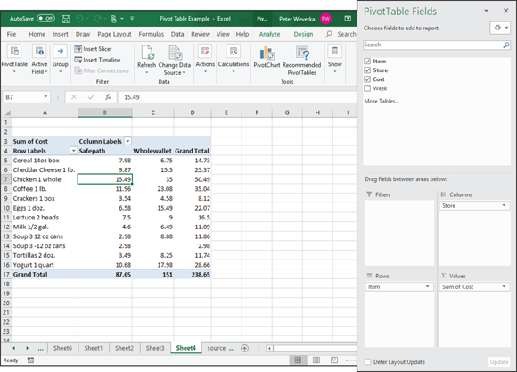
FIGURE 5-11: Constructing a PivotTable on the (PivotTable Tools) Analyze tab.

Putting the finishing touches on a PivotTable

Go to the (PivotTable Tools) Design tab to put the finishing touches on a PivotTable:

• Grand Totals: Excel totals columns and rows in PivotTables. If you prefer not to see these “grand totals,” click the Grand Totals button and choose an option to remove them from rows, columns, or both.
• Report Layout: Click the Report Layout button and choose a PivotTable layout on the drop-down list.
• PivotTable Styles: Choose a PivotTable style to breathe a little color into your PivotTable.

To construct a chart from a PivotTable, go to the (PivotTable Tools) Analyze tab and click the PivotChart button. The Insert Chart dialog box opens. Book 8, Chapter 1 explains how to navigate this dialog box.