Convolution
Pascal Wallisch
The purpose of this chapter is to familiarize you with the convolution operation. You will use this operation in the context of receptive fields in the early visual system as input response filters whose convolution with an input image approximates certain aspects of your perception. Specifically, you will reproduce the Mach band illusion and explore the Gabor filter as a model for the receptive field of a simple cell in the primary visual cortex.
Keywords
convolution; difference of Gaussians function; classical receptive field; Mach band illusion; excitatory; inhibitory
16.1 Goals of this Chapter
The purpose of this chapter is to familiarize you with the convolution operation. You will use this operation in the context of receptive fields in the early visual system as input response filters whose convolution with an input image approximates certain aspects of your perception. Specifically, you will reproduce the Mach band illusion and explore the Gabor filter as a model for the receptive field of a simple cell in the primary visual cortex.
16.2 Background
A convolution is the mathematical operation used to find the output y(t) of a linear time-invariant system from some input x(t) using the impulse response function of the system h(t), where h(t) is defined as the output of a system to a unit impulse input. It is defined as the following integral:
 (16.1)
This can be graphically interpreted as follows. The function h(τ) is plotted on the τ-axis, as is the flipped and shifted function x(t−τ), where the shift t is fixed. These two signals are multiplied, and the signed area under the curve of the resulting function is found to obtain y(t). This operation is then repeated for every value of t in the domain of y. It turns out that it doesn’t matter which function is flipped and shifted since h * x=x * h.
You can also define a convolution for data in two dimensions:
 (16.2)
Basically, you take a convolution in one dimension to establish the k dependence of the result y and then use that output (which is a function of k, t and τ) to perform another convolution in the second dimension. This second convolution provides the t dependence of the result, y. It is important that you understand how to apply this to a two-dimensional data function because in this chapter you will be working with two-dimensional images. In the MATLAB® software, since you are working with discrete datasets, the integral becomes a summation, so the definition for convolution in 2D at every point becomes
 (16.3)
Again, this is easier to understand pictorially. What you are doing in this algorithm is taking the dataset x, which is a matrix; rotating it by 180 degrees; overlaying it at each point in the matrix h that describes the response filter; multiplying each point with the underlying point; and summing these points to produce a new point at that position. You do this for every position to get a new matrix that will represent the convolution of h and x.
16.2.1 The Visual System and Receptive Fields
In this section we discuss in general the anatomy of the visual system and the input response functions that explain how different areas of the brain involved in this system might “perceive” a visual stimulus.
Light information from the outside world is carried by photons that enter the eyes and cause a series of biochemical cascades to occur in rods and cones of the retina. This biochemical cascade causes channels to close which leads to a decrease in the release of neurotransmitter onto bipolar cells. In general, there are two fundamental varieties of bipolar cells. On-bipolar cells become depolarized in response to light and off-bipolar cells become hyperpolarized in response to light. The bipolar cells then project to the ganglion cells which are the output cells of the retina. The response to light in this main pathway is also influenced by both the horizontal and amacrine cells in the retina. There are many types of retinal ganglion cells that respond to different visual stimuli.
A stimulus in the visual field will elicit a cell’s response (above the background firing rate) only if it lies within a localized region of visual space, denoted by the cell’s classical receptive field. In general, the ganglion cells have a center-surround receptive field due to the types of cells that interact to send information to these neurons. That is, the receptive field is essentially two concentric circles, with the center having an excitatory increase (+) in neuronal activity in response to light stimulus and the surround having an inhibitory decrease (−) in neuronal activity in response to light stimulus, or vice versa. The response function of the ganglion cells can then be modeled using a Mexican hat function, also sometimes called a difference of Gaussians function.
In the main visual pathway, the ganglion cells send their axons to the lateral geniculate nucleus (LGN) in the thalamus, which is in charge of regulating information flow to the cortex. These cells also are thought to have receptive fields with a center-surround architecture. LGN cells project to the primary visual cortex (V1). In V1, simple cells are thought to receive information from LGN neurons in such a way that they respond to bars of light at certain orientations and spatial frequencies. This can similarly be described as a Gabor function—a two-dimensional Gaussian filter whose amplitude is modulated by a sinusoidal function along an axis at a given orientation. Thus, different simple cells in V1 respond to bars of light at specific orientations with specific widths (this represents spatial frequency; see Dayan and Abbott, 2001). These and other cells from V1 project to many other areas in the cortex thought to represent motion, depth, face recognition, and other fascinating visual features and perceptions.
16.2.2 The Mach Band Illusion
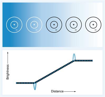
Using your knowledge of the receptive fields or the response functions of the visual areas can help you understand why certain optical illusions work. The Mach band illusion is a perceptual illusion seen when viewing an image that ramps from black to white. Dark and light bands appear on the image where the brightness ramp meets the black and white plateau, respectively. These bands are named after Ernst Mach, a German physicist who first studied them in the 1860s. They can be explained with the center-surround receptive fields of the ganglion or LGN cells (Ratliff, 1965; Sekuler and Blake, 2002); we will use this model in this chapter although alternative explanations exist (for example, see Lotto, Williams, and Purves, 1999).
The illusion is demonstrated in Figure 16.1. At the initiation of the stimulus brightness ramp, a dark band, darker than the dark plateau to the left, is usually perceived. At the termination of the brightness ramp, a light band is perceived brighter than the light plateau to its right. Figure 16.1 shows the center-surround receptive fields of sample neurons, represented by concentric circles, superimposed on the stimulus image. The center disk is excitatory, and the surrounding annulus is inhibitory, as indicated by the plus and minus signs. When the receptive field of a neuron is positioned completely within the areas of uniform brightness, the center receives nearly the same stimulation as the surround; thus, the excitation and inhibition are in balance. A receptive field aligned with the dark Mach band has more of its surround in a brighter area than the center, and the increased inhibition to the neuron results in the perception of that area as darker. Conversely, the excitation to a neuron whose receptive field is aligned with the bright Mach band is increased, since more of its center is in a brighter area than the surround. The decreased inhibition to such a neuron results in a stronger response than that of the neuron whose receptive field lies in the uniformly bright regime and thus the perception of the area as brighter.
16.3 Exercises
The goal for this chapter is to reproduce the Mach band optical illusion. First, you will create the visual stimulus. Then you will create a center-surround Mexican hat receptive field. Finally, you will convolve the stimulus with the receptive field filter to produce an approximation of the perceived brightness.
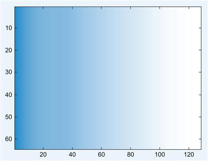
You begin by creating the M-file named ramp.m that will generate the visual input (see Figure 16.2). The input will be a 64×128 matrix whose values represent the intensity or brightness of the image. You want the brightness to begin dark, at a value of 10, for the first 32 columns. In the next 65 columns, the value will increase at a rate of one per column, and the brightness will stay at the constant value of 75 for the rest of the matrix. Open a new blank file and save it under the name ramp.m. In that file enter the following commands:
% This script generates the image that creates the Mach band visual illusion.
In=10*ones(64,128); %initiates the visual stimulus with a constant value of 10
%ramps up the value for the middle matrix elements (column 33 to column 97)
In(:,98:end)=75; %sets the last columns of the matrix to the final brightness value of 75
imagesc(In); colormap(bone); set(gca, ‘fontsize’,20) %view the visual stimulus
Notice how the function imagesc creates an image whose pixel colors correspond to the values of the input matrix In. You can play with the color representation of the input data by changing the colormap. Here, you use the colormap bone, since it is the most appropriate one for creating the optical illusion, but there are many more interesting options available that you can explore by reading the help file for the function colormap.
You’ve just created an M-file titled ramp that will generate the visual stimulus. Note, however, that you use a for loop in ramping up the brightness values. Although it doesn’t make much of a difference in this script, it is good practice to avoid using for loops when programming in MATLAB if possible, and to take advantage of its efficient matrix manipulation capabilities for faster run times (see Chapter 4.4.5.1, “Vectorizing Matrix Operations”). How might you eliminate the for loop in this case? One solution is to use the function cumsum. Let’s see what it can do:
The function will cumulatively add the elements of the matrix by row, unless you specify that dimension along which to sum should be the second dimension, or by column:
You will want this cumulative sum by columns for this ramp function. Now rewrite the code in proper style for MATLAB without the for loop:
% This script generates the image that creates the Mach band visual illusion.
In=10*ones(64,128); %initiates the visual stimulus with a constant value of 10
% now ramp up the value for the middle matrix elements using cumsum
In(:,33:97)=10+cumsum(ones(64,65),2);
In(:,98:end)=75; %sets the last columns of the matrix to the end value of 75
figure; imagesc(In); colormap(bone); set(gca, ‘fontsize’,20) %view the visual stimulus
You can look at how the values of the brightness increase from left to right by taking a slice of the matrix and plotting it, as shown in Figure 16.3. Look at the 32nd row in particular.
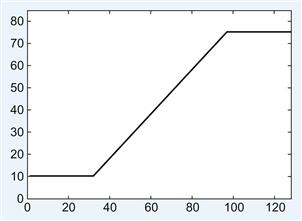
Figure 16.3 The brightness values in a slice through the ramp stimulus shown in Figure 16.2.
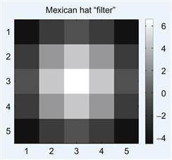
Next, you will create a script titled mexican_hat.m that will generate a matrix whose values are a difference of Gaussians. For this exercise, you will make this a 5×5 filter, as shown in Figure 16.4.
% this script produces an N by N matrix whose values are
% a 2 dimensional Mexican hat or difference of Gaussians
IE=6; %ratio of inhibition to excitation
Se=2; %variance of the excitation Gaussian
Si=6; %variance of the inhibition Gaussian
S = 500;%overall strength of Mexican hat connectivity
[X,Y]=meshgrid((1:N)-round(N/2));
% −floor(N/2) to floor(N/2) in the row or column positions (for N odd)
% −N/2+1 to N/2 in the row or column positions (for N even)
% Switch from Cartesian to polar coordinates
% R is an N*N grid of lattice distances from the center pixel
% i.e. R=sqrt((X).^2 + (Y).^2)+eps;
EGauss = 1/(2*pi*Se^2)*exp(-R.^2/(2*Se^2)); % create the excitatory Gaussian
IGauss = 1/(2*pi*Si^2)*exp(-R.^2/(2*Si^2)); % create the inhibitory Gaussian
MH = S*(EGauss-IE*IGauss); %create the Mexican hat filter
figure; imagesc(MH) %visualize the filter
Now take a second look at some of the components of this script. The function meshgrid is used to generate the X and Y matrices whose values contained the x and y Cartesian coordinate values for the Gaussians:
The function cart2pol converts the Cartesian coordinates X and Y into the polar coordinates R and THETA. You use this function to create the 5×5 matrix R whose values are the radial distance from the center pixel:
2.8284 2.2361 2.0000 2.2361 2.8284
2.2361 1.4142 1.0000 1.4142 2.2361
The THETA variable is never used; however, it gives the polar angle in radians:
−2.3562 −2.0344 −1.5708 −1.1071 −0.7854
−2.6779 −2.3562 −1.5708 −0.7854 −0.4636
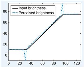
Finally, you’re ready to generate the main script called mach_illusion.m to visualize how the Mexican hat function/center-surround receptive field of the neurons in the early visual system could affect your perception. In this simple model, the two-dimensional convolution of the input image matrix (generated by the ramp.m M-file) with the receptive field filter (generated by the mexican_hat.m M-file) gives an approximation to how the brightness of the image is perceived when filtered through the early visual system. This operation should result in a dip in the brightness perceived at the point where the brightness of the input just begins to increase and a peak in the brightness perceived at the point where the brightness of the input just stops increasing and returns to a steady value, consistent with the perception of Mach bands (see Figure 16.5). For a first pass, use the two-dimensional convolution function, conv2, that is built into MATLAB. As described in detail in the help section, this function will output a matrix whose size in each dimension is equal to the sum of the corresponding dimensions of the input matrices minus one. The edges of the output matrix are usually not considered valid because the value of those points have some terms contributing to the convolution sum which involved zeros padded to the edges of the input matrix. One way to deal with the problem of such edge effects is to reduce the size of the output image by trimming the invalid pixels off the border. You accomplish this by including the option ‘valid’ when calling the conv2 function:
mexican_hat %creates the Mexican hat matrix, MH, & plots
ramp %creates image with ramp from dark to light, In, & plots
A=conv2(In,MH,’valid’); %convolve image and Mexican hat
figure; imagesc(A); colormap(bone) %visualize the "perceived" brightness
%create plot showing the profile of both the input and the perceived brightness
figure; plot(In(32,:),’k’,’LineWidth’,5); axis([0 128 −10 95])
hold on; plot(A(32,:),’b-.’,’LineWidth’,2); set(gca,’fontsize’,20)
lh=legend(‘input brightness’,’perceived brightness’,2); set(lh,’fontsize’,20)
Make sure that the mexican_hat.m and ramp.m M-files are in the same directory as the mach_illusion.m M-file. Note that the size of the output is indeed smaller than the input:
For fun, you can learn more about how the convolution works by changing the ‘valid’ option in the conv2 function call to either ‘full’ or ‘same’ and see how the output matrix A changes. One way to minimize the edge effects of convolution is to pad the input matrix with values that mirror the edges of the input matrix before performing the two-dimensional convolution and returning only the valid part of the output, which will now be the size of the original input matrix. The function conv2mirrored.m will do just this trick. It has been written in a generic form to accept matrices of any size:
function sp = conv2_mirrored(s,c)
% 2D convolution with mirrored edges to reduce edge effects
% output of convolution is same size as leading input matrix
[n,m]=size(c); %% both n & m should be odd
% enlarge matrix s in preparation for convolution with matrix c
%via mirroring edges to reduce edge effects.
sp=[zeros(padn,M+(2*padm)); zeros(N,padm) s zeros(N,padm); zeros(padn,M+(2*padm))];
sp(1:padn,:)=flipud(sp(padn+1:2*padn,:));
sp(padn+N+1:N+2*padn,:)=flipud(sp(N+1:N+padn,:));
sp(:,1:padm)=fliplr(sp(:,padm+1:2*padm));
16.4 Project
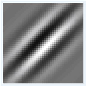
The receptive fields of simple cells in V1 reflect the orientation and spatial frequency preference of the neurons. One way to model this is to use the Gabor function, which is basically a two-dimensional Gaussian modulated by a sinusoid, as shown in Figure 16.6.
1. Observe how the receptive fields of simple cells in V1 modeled as Gabor functions with various spatial frequency and orientation preferences filter an image of a rose, which can be downloaded from the companion web site. Create two files, the gabor_filter.m function and the gabor_conv.m script (using the following code), in the same directory as the conv2_mirrored.m file. Also, place the rose.jpg image file in the same directory. Now, run the gabor_conv.m script. It will take a convolution between the rose image with a Gabor function of a given orientation (OR) and spatial frequency (SF). The input parameters OR and SF will determine the orientation and spatial frequency of the filter. Thus, you will essentially “see” how simple cells in V1 with a given orientation and spatial frequency preference perceive an image. Try values of SF=0.01, 0.05, and 0.1, and OR=0, pi/4, and pi/2. Put the resulting figures into a document and explain the results. Try changing the Gabor filter from an odd filter to an even filter by using cos instead of sin. How does this affect the output?
function f = gabor_filter(OR, SF)
% Creates a Gabor filter for orientation and spatial frequency
% selectivity of orientation OR (in radians) and spatial frequency SF.
sigma_x=7;% standard deviation of 2D Gaussian along x-dir
sigma_y=17;% standard deviation of 2D Gaussian along y-dir
X=x*cos(OR)+y*sin(OR); %rotate axes
f=(1/(2*pi*sigma_x*sigma_y)).*exp(-(1/2)*(((X/sigma_x).^2)+...
((Y/sigma_y).^2))).*sin(2*pi*SF*X);
subplot(1,3,1); imagesc(G); axis square; colorbar; title (‘Gabor function’)
subplot(1,3,2); imagesc(I); title(‘original image’)
subplot(1,3,3); imagesc(conv2_mirrored(double(I),G));
colormap(bone); title([‘Convolved image OR=‘,num2str(OR),’ SF=‘, num2str(SF)])
2. Now you can have some fun times with image processing and convolutions. Choose any image and convolve it with a function or filter of your choosing. To avoid edge problems, you can use the conv2_mirrored function provided, the conv2 function with the ‘valid’ option (as in the exercises), or you can use the function imfilter from the Image Processing Toolbox built into MATLAB, which does an operation similar to convolution. You can create your own filter or choose a predesigned filter in MATLAB using the fspecial function, also from the Image Processing Toolbox. You can learn more about these functions through the online help. Hand in your code and picture of before and after the filtering, along with an image of the filter used in the convolution.
