Fitzhugh-Nagumo Model
Traveling Waves
Pascal Wallisch
The purpose of this chapter is to learn how to model traveling waves in an excitable media. This entails the solution of a partial differential equation involving a first derivative in time coordinates and a second derivative in spatial coordinates. You will learn how to compute a second derivative in the MATLAB® software, and use a modification of the Fitzhugh-Nagumo model to generate traveling waves in both one and two dimensions.
Keywords
reaction-diffusion equation; Fitzhugh-Nagumo model; centered second difference; periodic boundary conditions; free boundary conditions; ordinary differential equation solver
30.1 Goals of This Chapter
The purpose of this chapter is to learn how to model traveling waves in an excitable media. This entails the solution of a partial differential equation involving a first derivative in time coordinates and a second derivative in spatial coordinates. You will learn how to compute a second derivative in the MATLAB® software, and use a modification of the Fitzhugh-Nagumo model introduced in Chapter 15, “Exploring the Fitzhugh-Nagumo Model,” to generate traveling waves in both one and two dimensions.
30.2 Background
The Fitzhugh-Nagumo model is often used as a generic model for excitable media because it is analytically tractable. You will use it as a simple model to generate traveling waves by the addition of a diffusion term: a second derivative in spatial coordinates. In this chapter, you will modify the Fitzhugh-Nagumo model introduced in Chapter 15 in this way, and study its behavior in one and two dimensions. Thus you can simulate action potential wave propagation along the axon of a single neuron or the spreading of electrical potential waves in a network of cortical neurons.
There are many forms of the equations for the voltage, v, and recovery, r, variables in the Fitzhugh-Nagumo model. In general they are given by:
 (30.1)
 (30.2)
The function f(v) is a third order polynomial that provides positive feedback, whereas the slower recovery variable r provides negative feedback. By making the voltage and recovery variables functions of spatial coordinates as well as time, you can model dynamics in a spatially extended regime. The final term in the first equation introduces diffusion into the system, and thus the first equation is known as a reaction-diffusion equation.
A note of caution: As with ordinary differential equations, whenever you attempt to solve partial differential equations computationally, you must be careful that the various errors that can be introduced, such as truncation errors and roundoff errors, are not significant and that the necessary conditions for stability are met. See Strauss (1992) for a more in-depth discussion of such matters. If you are not careful, then the solutions produced by your code may stray quite significantly from the true solutions you seek.
30.3 Exercises
30.3.1 Second Derivative Operator
How do you model a second derivative computationally in MATLAB? There are a few approaches to this, but the one you will use here is the simplest computational approximation known as the centered second difference:
 (30.3)
This approach can be justified by combining the Taylor expansions for v(x+Δx) and v(xΔx) (Strauss, 1992). If the mesh size of the spatial variable is represented by Δx, then the jth element of the array v, vj, is the value of v for x=jΔx, so you have:
 (30.4)
The second derivative can thus be computed by convolving the array v with the second derivative operator filter F=[1 −2 1]/(Δx)2. This can be extended to two dimensions as well. Assuming equal mesh spacing along both directions (Δx=Δy), then the two-dimensional second derivative operator filter is given by F=[0 1 0; 1 −4 1; 0 1 0]/(Δx)2.
Now create a function in MATLAB for the second derivative operator in one dimension, and name it secDer.m. Its input will be the one-dimensional array v(x) and the spatial mesh size, dx, and the output will be the second derivative, v’’(x). This function will use the convolution function conv, which, by default, introduces undesirable edge effects. Also include an option to improve the edge effects by making the boundary conditions periodic. You’ll do this by adding a third input to the function, BC, which, if set to 1, will return the default conv output found by padding the input matrix with zeros, also known as free boundary conditions, and if set to 2, then you will have periodic boundary conditions. Periodic boundary conditions means that the boundaries of the input array (i.e., the first and last elements) are considered neighboring points. You could use the if, elseif control structure to carry out the options for the boundary conditions, but instead we will introduce you to another useful control structure that MATLAB offers: switch.
%F is the discrete 2nd derivative filter in 1D
%BC determines your boundary conditions
V=V(2:end-1); %return an array the same size as the input array
%since the convolution filter is of length 3 then we only have to
%pad the input array v by 1 element on either side
pv=zeros(1,length(v)+2); %extend the input array by 2
%now we fill in these two padded points with the values that the extended
%input array would have if the first element of v and the last element of v
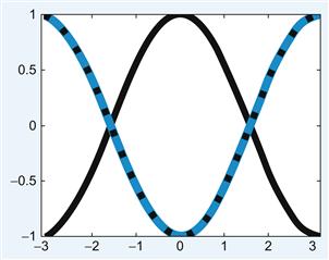
Give this a try and see how it works by testing it on a function whose second derivative is well known: cosine. If f(x)=cos(x), then f’’(x) = -cos(x). You can compare the output of the second derivative function, secDer, with the analytic solution by running the following script, whose output is shown in Figure 30.1.
x=linspace(-pi,pi,100); %forces even spacing in array of 100 pts from –pi to pi
dx=x(2)-x(1); %determines this spacing, the spatial mesh size
x=x(2:end); % for periodicity knock of 1st term in x array so that we don’t have repeat % value of cos(x) at the endpoints of x (since cos(-pi)=cos(pi))
d2f=secDer(f,dx,2); %computational solution to the second derivative
d2fA=-cos(x); %analytic solution to the second derivative of f
plot(x,f,‘k’,‘LineWidth’,3) %plot input f
plot(x,d2f,‘b’,‘LineWidth’,5) %plot computational result of f"

Figure 30.1 Testing the second derivative function secDer.m. The solid black line is the input, cos(x), and the blue line is the output of the secDer function with periodic boundary conditions. This matches exactly with the analytic solution to the second derivative, -cos(x), shown as the dotted black line.
With this second derivative operator, you can now model a traveling wave in 1D. For the one-dimensional problem, you will use the following form of the Fitzhugh-Nagumo equations (Wilson, 1999):
 (30.5)
 (30.6)
The variables v(x,t) and r(x,t) are the voltage and the recovery variables at position x at time t. If modeling a pulse traveling along a nerve fiber, you can think of x as the position along the nerve fiber. Similarly, if you want to model a traveling wave of activity across a one-dimensional network of neurons, then x indicates the neuron location in the one-dimensional population. Now consider the latter case. You will use the following parameter values: D=1, a=1.5, b=1, and p=0.8. For this set of parameters, the steady state values are v0=–1.5 and r0=–3/8, which you will use as your initial conditions for these variables. The driving stimulus is given by I. To solve this system, you are going to need an ODE solver.
30.3.2 Built-in ODE Solvers
In previous chapters, you solved differential equations through manually written ODE solvers using the Euler method and the Runge-Kutta method, which had the advantage of complete transparency in the mechanisms behind the operations. In this chapter, we will introduce you to the most practical and commonly used of the built-in ODE solvers in MATLAB: the function ode45. This solver is based on an explicit Runge-Kutta formula and has been optimized to adaptively find the most efficient time steps to produce a solution within a certain allowed relative error tolerance (10−3 by default) and absolute error tolerance (10−6 by default). Look at the help section for ode45 for more information on how to adjust these options as well as to learn about the other built-in ODE solvers offered by MATLAB and the conditions under which to use them.
To familiarize yourself with the proper syntax for using the ode45 ODE solver, first consider the simpler case of solving this system of equations for one point in space (i.e., for one neuron). First, you must code the system of first-order ODEs as a function that the solver can use. You will represent the Fitzhugh-Nagumo system in a function called F_N1. The F_N1 function assumes that v and r become elements V(1) and V(2) of the two-element input vector V. Although t and V must be the function’s first two arguments, the function does not need to use them. The output vdot, the derivative of V, must be a column vector, as shown in the following code:
vdot(1) = 10*(V(1) - (V(1).^3)/3 - V(2) + I);
vdot(2) = p*(1.25*V(1) + a – b*V(2));
vdot=vdot’; %make correct dimensions for ODE solver: must be a column vector
Note that the diffusion term is left out, since there is only one point in space and a spatial derivative makes no sense in this case. For this one neuron system, you set the input to 1.5 so that the model will initiate a series of action potentials. You can then generate and plot the solution as follows:
v0=[−1.5;−3/8]; %initial conditions for V variable
tspan=[0 100]; %beginning and end values of time
Now look at what was produced by running the preceding script:

Note that the time, which goes from 0 to 100, is a column vector of 2597 points. These time points are not evenly distributed between 0 and 100; rather, the mesh size varies and has been selected by the solver to most efficiently compute the differential equation within the tolerated error. For example, consider how the spacing between time points varies in just the first 10 time points:
The first column of the output vector, v(:,1), represents the voltage values at the corresponding times starting with v0(1) at the first time point. Similarly, the second column of the output vector, v(:,2), represents the recovery variable values for the corresponding times, starting with v0(2).
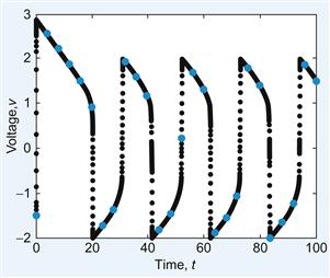
When you specify specific time points in tspan, the ODE solver will still use its most efficient time mesh to solve the differential equation; however, it will now return the values of the outputs at the specific times indicated in tspan. Compare the previous result with that found by specifying the time to be from 0 to 100 at intervals of 4:
This result is shown in Figure 30.2.
30.3.3 Fitzhugh-Nagumo Traveling Wave
You are now ready to tackle the full problem of simulating a propagating wave along a line of neurons. Let the number of neurons be given by N. A naïve approach might be to allow the initial conditions to be a 2×N matrix with the first row representing the N initial voltages and the second row the N values of the initial recovery variables. However, recall that the ode45 solver will accept only a single column array for the initial conditions. What you will do to satisfy this requirement is let the initial value column vector be of length 2N and let the first N elements represent the initial voltages of the N neurons and the last N elements represent the initial recovery values. The ODE solver will produce as its output a t×1 time vector, and a t×2N matrix, whose first N columns represent the evolution of the voltage of the population of neurons as time progresses and whose second N columns represent the evolution of the recovery variables.
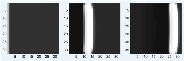
The stimulus to initiate the wave that you will use is I=6 for the first 0.5 s; then the stimulus will be off, I=0, for the rest of the time. You can choose where along the line of neurons to initiate the wave. In the following example, you stimulate the center cells. The following script, FNmain.m, will produce a traveling wave of activity along a one-dimensional population of N neurons whose dynamics are governed by the Fitzhugh-Nagumo equations, as shown in Figure 30.3.
global N I BC %by making these variables global they can exist within
%the workspace of functions without explicitly being input to the functions
v0(1:N)=−1.5; %initial conditions for V variable
v0(N+1:2*N)=−3/8; %initial conditions for R variable
I=6; %the input stimulus value
BC = 2; %set to 1 (free) or 2 (periodic boundary conditions)
tspan=[0:.1:.5]; %time with stimulus
[t1,v1] = ode45(‘F_N’,tspan,v0);
tspan=[.5:.1:25]; % time without stimulus
[t2,v2] = ode45(’F_N’,tspan,v1(end,:)’); %note: initial cond are final v1 values
%piece together (concatenate) time (t1 and t2) and solution (v1 and v2)
%variables without double counting the seam values
t=[t1; t2(2:end)]; v=[v1; v2(2:end,:)];
%spacetime plot of v variable w/ neurons along y axis, time along x-axis
figure(1); imagesc(v(:,1:N)’) ; colorbar
%spacetime plot of r variable w/ neurons along y axis, time along x-axis
figure(2); imagesc(v(:,N+1:end)’); colorbar

Figure 30.3 Traveling Fitzhugh-Nagumo wave in one dimension for t=1 (left), t=5 (center), and t=10 (right).
When you run the preceding FNmain.m script, make sure that this M-file is in the same directory as the secDer function previously created as well as the following function F_N, since the main script calls these functions. The function F_N describes the coupled system of differential equations used to model the dynamics.
vdot(1:N) = 10*(v(1:N) - (v(1:N).^3)/3 - v(N+1:end)) + D*secDer(v(1:N),1,BC)’;
%add input I to the center five cells
vdot(round(N/2)-2:round(N/2)+2) = vdot(round(N/2)-2:round(N/2)+2) + I;
30.4 Project
In this project, you will simulate a traveling wave of activity in a two-dimensional N×N array of cortical neurons. This time you will use these versions of the Fitzhugh-Nagumo equations (Murray, 2002):
 (30.7)
 (30.8)
with the parameters taking on the values a=0.25, b=0.001, g=0.003, and D=0.05. You will compute the solution using a similar method as that used for the one-dimensional problem. This time the initial value column vector will be of length 2N2, where the first N2 elements will represent the initial voltages of the N×N neuron array and the last N2 elements will represent the initial recovery values. The ODE solver will produce as its output a t×1 time vector, and a t×2N2 matrix, whose first N2 columns represent the evolution of the voltage of the population of neurons as time progresses and whose second N2 columns represent the evolution of the recovery variables. For a given row of this output matrix, i.e., a particular time point, you can reconstruct the N×N array of voltage variables from the 1×N2 array using the reshape function, whose input is the matrix to be reshaped as well as the number of rows and columns desired in the output.
You will need to do this when you call the two-dimensional second derivative function as well as when you wish to visualize the results. There are more elegant and efficient ways to handle the issue of programming the two-dimensional partial differential equation, but here we will present a way to solve the problem in MATLAB that is conceptually simple, allowing you to use the tools previously used while not introducing any more complicated commands.
In the following script, FN2main.m, you will create an .avi file of the simulation and name it TravelingWave.avi:
% next 4 lines are to create the movie file of the wave
set(gca,‘NextPlot’,‘replace’,‘Visible’,‘off’)
mov = avifile(‘TravelingWave.avi’)
tspan=[0:5:800]; %simulation time
BC=1; %boundary conditions: 1 free, 2 periodic
v0(1:N^2)=0; %initial conditions for V variable
v0(N^2+1:2*N^2)=0; %initial conditions for R variable
v0(1:N) =.6; %initially stimulate all cells along left edge of population
[t,v] = ode45(‘F_N2’,tspan,v0);
%obtain min and max values of output
clims = [min(min(v(:,1:N^2))) max(max(v(:,1:N^2)))];
%generate the movie of the voltage
Specifying the same clims in the imagesc option for each time frame of the imaged voltage array ensures that the same colormap is used throughout the movie, which is analogous to using consistent z-axis limits. The preceding main script calls on a number of functions that need to be created and stored in the same directory as the main script. These functions, F_N2, SecDer2, and conv2periodic, follow. Note that you will need to complete the F_N2 function. The SecDer2 function is just an extension of the SecDer function to two dimensions and employs the reshape function to carry out the 2D convolutions. The conv2_periodic function has been written in a generic form so that it can handle input matrices of various sizes for future applications.
D=.05; a=0.25; b=.001; g=.003; %set the parameters
vdot(1:N^2)=-(v(1:N^2)).*(a-(v(1:N^2))).*(1-(v(1:N^2)))-...
v(N^2+1:end)+D.*secDer2(v(1:N^2),1,BC);
F = [0 1 0; 1 −4 1; 0 1 0]/dx^2;
%determines your boundary conditions
V=conv2(reshape(v,N,N)’,F,‘same’);
V=conv2_periodic(reshape(v,N,N)’,F);
function sp = conv2_periodic(s,c)
% 2D convolution for periodic boundary conditions.
% Output of convolution is same size as leading input matrix
[n,m]=size(c); %% both n & m should be odd
%enlarge matrix s in preparation convolution with matrix c via periodic edges
sp=[zeros(padn,M+(2*padm)); ...
zeros(NN,padm) s zeros(NN,padm); zeros(padn,M+(2*padm))];
%fill in zero padding with the periodic values
sp(1:padn,padm+1:padm+M)=s(NN+1-padn:NN,:);
sp(padn+1+NN:2*padn+NN, padm+1:padm+M)= s(1:padn,:);
sp(padn+1:padn+NN,1:padm)= s(:,M+1-padm:M);
sp(padn+1:padn+NN,padm+M+1:2*padm+M)= s(:,1:padm);
sp(1:padn,1:padm)= s(NN+1-padn:NN,M+1-padm:M);
sp(padn+NN+1:2*padn+NN,1:padm)= s(1:padn,M+1-padm:M);
sp(1:padn,padm+M+1:2*padm+M)=s(NN+1-padn:NN,1:padm);
sp(padn+NN+1:2*padn+NN,padm+M+1:2*padm+M)=s(1:padn,1:padm);
In this project, you should do the following:
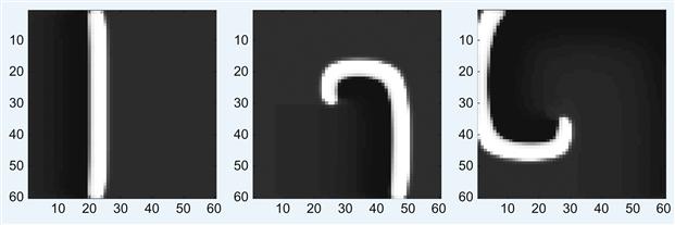
1. Create the main script and the functions given here in the same working directory. Complete the F_N2 function by replacing the symbols ??? with the proper quantities so that F_N2 implements the Fitzhugh-Nagumo model equations as given in this section. Run the main script to generate a plane wave from the left, as shown in Figure 30.4.
2. Alter the code so that the wave is initiated from one of the corners or in the center of the array and forms a propagating ring. Also try running the simulation with periodic boundary conditions. Play with the various parameters to see how they affect the wave dynamics.
3. Now use the model to generate a spiral by resetting the upper half of the voltage and recovery variables to 0 when the traveling plane wave is approximately halfway across the neural network. Start with the original code, as in the first part of the project so that a plane wave is initiated along the entire left edge of the array. In the main script, change the name of the .avi file that will be created to SpiralWave.avi. Let N=60 and tspan=[0:5:1800]. This will cause the simulation to take more time to run but will allow you to view the spiral well.
In the main script, create a variable Reset that can take on the value 0 or 1. Use the switch control structure so that when Reset is equal to 0, it runs the original script, and when it is equal to 1, the line [t,v] = ode45(‘F_N2’,tspan,v0); will not be executed, and in its place the following lines will be executed:
[t,v] = ode45(‘F_N2’,tspan,v0);
[t1,v1] = ode45(‘F_N2’,tspan(1:round(length(tspan)/3)),v0);
[t2,v2] = ode45(‘F_N2’,tspan(round(length(tspan)/3):end),vR);
Create the following Vreset function in the same directory as the main file:
%reset half of voltage variables to zero
%reset half of recovery variables to zero
RR = reshape(v(N^2+1:end),N,N)’;
vR=[reshape(VR’,N*N,1);reshape(RR’,N*N,1)];
Explain how the Vreset function works. Submit the main script and set of functions that give the option to generate spiral waves. Plot screenshots of the spiral wave generated at various timesteps t(i) by using the command:
imagesc(reshape(v(i,1:N^2),N,N), clims); axis square
for various values of i, as shown in Figure 30.5. Again, you can play with the various parameters to see how they affect the wave dynamics.


