Modeling Spike Trains as a Poisson Process

This chapter focuses on point process models for characterizing and simulating trains of actions potentials generated by neurons. Initially, a simple homogeneous Poisson process model will be introduced to capture fundamental characteristics. Models with greater sophistication will be introduced to incorporate more complex activity, such as refractory periods and bursting.

Keywords

Poisson process model; event train; Bernoulli process; probability density function; scalar; Poisson distribution

33.2 Background

Often when attempting to characterize extracellular activity, plausible values for simulating the underlying intracellular phenomena driving the activity are not available. In such cases, a stochastic description of the observed activity can be a useful model for the event train produced by the cell.

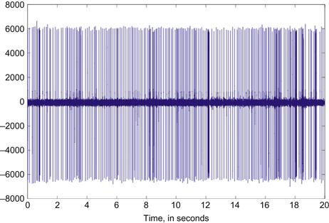
Consider the spike train in Figure 33.1. How can the sequence of neural events be characterized? A very simple characterization is the mean event rate per unit time. In this case, that value is 11.3 ips. This value has the advantage of being a scalar: easily computed and easily manipulated. However, reducing all the activity in a spike train to a single number discards any temporal structure in the events.

Figure 33.1 An extracellularly recorded spike train.

Still, even a simple characterization can lead to useful insights. If we choose a temporal interval substantially smaller than the mean rate, we can treat the mean rate as an event probability during that event. Such a model, with discrete intervals of time, is described by a Bernoulli process.

33.3 The Bernoulli Process: Events in Discrete Time

A Bernoulli process generates a sequence of event times corresponding to positive events from a series of Bernoulli trials. However, in a Bernoulli process, time is measured discretely, so that the event “time” is the index of the corresponding discrete time interval. Each discrete interval corresponds to a Bernoulli trial with probability p of success or 1−p of failure. For example, taking heads as a success, a sequence of coin tosses in which the time intervals of the successful (i.e., heads) tosses are noted constitutes a Bernoulli process.

Taking each time interval as a trial, we can treat the simple model just described as a Bernoulli process.

Exercise 33.1

Use a Bernoulli process to simulate a spike train from the mean activity rate for the spike train in Figure 33.1. Take the mean rate of 11.3 ips, and use a time slice of 1 ms. Generate a 20 s train (i.e., 20,000 time slices). Treat each time slice as a Bernoulli random variable with a small probability of a neural event. The p value (probability of an event) should be chosen so that the mean successes over 1000 trials equals the mean rate, or Np= 11.3 events, where N is the number of time slices in one second. A success will correspond to a neural event occurring during the time slice. To pick a uniform random number between 0 and 1, rand can be used:

0.9134 0.0975
0.6324 0.2785

Unfortunately, the Bernoulli process falls short in some important ways. Most importantly, as mentioned earlier, the Bernoulli process is discrete: a consequence of this is that the event times are no more precise than the time interval. Looking at a distribution of the interspike intervals with a bin size smaller than the time interval used for the Bernoulli process illustrates this quite clearly. Fortunately, there is an analogous process for continuous time: the Poisson process. Exploring the Poisson process will be the focus of the next section.

33.4 The Poisson Process: Events in Continuous Time

Like the Bernoulli process, a Poisson process is a counting process (i.e., the event count increases with increasing time), but instead of counting discrete events, a Poisson process describes events in continuous time.

A Poisson process adheres to the following criteria:

1. Event counts in disjoint intervals are statistically independent, and depend only on the size of the interval.

2. No two events occur simultaneously.

From these simple properties, the form of the Poisson distribution can be derived. Below is the probability mass function for the Poisson distribution.

A Poisson distribution is parameterized by a single value, lambda. Lambda is often interpreted as the rate of success. This interpretation falls out of the expectation of the distribution.

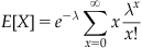
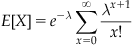
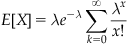
The term on the far right hand side is the Taylor expansion at 0 for , which when multiplied by the adjacent cancels, leaving

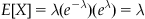
as the expectation. In other words, the mean event count of a Poisson distribution with value lambda is lambda. The parameter lambda can also be interpreted as the mean event count over an interval T, for which λ can be written as λ=rT. When expressed as the mean event count over an interval of length T, r represents the mean event count per unit interval. Thus, for an interval , the corresponding lambda is .

From the criteria above, the distribution of time intervals between events can be shown to follow an exponential distribution. Unlike the Poisson distribution of event counts, the exponential distribution is a continuous distribution, with probability density function (PDF) instead of a probability mass function. Here is the PDF for an exponential distribution with parameter λ:

Exercise 33.2

Demonstrate that the variance of the Poisson distribution is the same as the mean, λ. Demonstrate that the mean of the exponential distribution is .

It should be noted that while the distribution of time intervals between consecutive events follows an exponential distribution, the distribution of event times follows a uniform distribution. This implies that any one event is no more probable at one time than any other.

33.4.1 Simulating an Event Train Using a Poisson Model

Here, we will introduce two approaches for simulating an event train with a Poisson model. A simple approach is to draw intervals between consecutive events from an exponential distribution. This approach works quite well when needing to generate consecutive events without an explicit time bound.

Alternatively, one can use a different approach if working with a fixed time bound. Building on the principle that event times are uniformly distributed, one can draw a sample event count for the interval from an appropriate Poisson distribution, and then draw times for each event by picking from an appropriate random distribution for each event.

1. Take an interval T and a rate r

2. Draw a sample event count N for interval T from a Poisson distribution with parameter λ=Tr

3. Draw N times, t₁, t₂, t₃, … t_N, from a uniform distribution ranging from 0 to T

4. Return t₁, t₂, t₃, … t_N as the event times.

33.4.2 Picking Poisson and Exponentially Distributed Values

In most cases, the Statistics Toolbox will be available. The Statistics Toolbox offers a wide selection of functions to calculate probability density functions, cumulative distribution functions, inverse cumulative distribution functions, and generate random variables. Naming conventions for various distributions typically add a suffix denoting the type of calculation, such as cumulative distribution function or random variable generation, to an abbreviated name of the distribution. For example, here are functions for the Poisson distribution:

poissrnd—Poisson distributed random variables

poisspdf—Poisson probability density function

poisscdf—Poisson cumulative distribution function

poissinv—inverse Poisson cumulative distribution function

Exercise 33.3

Demonstrate that both methods of generating event trains produce similarly distributed values. For each method, generate at least 5 minutes of event data for a cell with a mean rate of 10 ips. Compare empirical distributions of ISI and event counts per second. The Statistics Toolbox provides the functions poissrnd, exprnd, and unifrnd to draw from Poisson, exponential, and uniform distributions respectively.

(If the Statistics Toolbox is not available, see the next section for alternatives.)

33.5 Picking Random Variables Without the Statistics Toolbox

If the Statistics Toolbox is not available, there are a number of methods for drawing exponential and Poisson distributed random variables using only a uniformly distributed random variable between 0 and 1. The MATLAB® function rand, introduced earlier, is not part of the Statistics Toolbox and should be available under even a basic installation.

33.5.1 Exponential Distributions

A simple method for generating values with an exponential distribution, the inversion method, relies on the uncomplicated form of the inverse of the cumulative probability function. For a given value of a random variable, the cumulative probability function returns the probability that a random variable will be less than the given value. The cumulative probability function is calculated from the probability density function f(x) through the integral

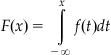
The cumulative probability function maps a value of the distribution to a probability. The inverse of the cumulative probability function maps a probability to a corresponding random variable in the distribution. With an inverse cumulative probability function and a uniform distribution from 0 to 1, we can generate exponentially distributed values (this is actually valid for any inverse cumulative probability function).

The inverse cumulative function takes the form

where U is uniformly distributed over 0…1.

Exercise 33.4

Derive the inverse cumulative probability function from the probability density function. Hint: the quantity 1−U, where U is a uniformly distributed random variable from 0…1, is itself also a uniformly distributed random variable from 0…1.

To generate the next event time for a Poisson process with parameter λ:

1. Select a random value, U, uniformly distributed from 0…1

2. Calculate Δt=−(ln U)/λ (This is the interval between events, not the event time itself!)

3. Return event time t_n=t_n−1+Δt

The following MATLAB function implements the above algorithm, generating a valid time for the next event given a lambda value and the time of the previous event.

function t = next_event(lambda, event)

U = rand;

dt = -log(U)/lambda;

t = event + dt;

end

33.5.2 Poisson Distributions

If a viable generator for exponentially distributed variates is available, successive exponential values can be generated until the combined time exceeds the interval over which a Poisson trial is needed. Then, the Poisson success count is the number of exponential variables whose summed time is less than the interval.

1. Start with parameter lambda, λ, the interval T

2. Let T′, the cumulative time, and N, the event count, be set to 0

3. Select t, an exponentially distributed interval with parameter λ

4. If T′+t > T, return N as the number of events in the interval

5. T′=T′+t

6. N=N+1

The inversion method (i.e., using the inverse cumulative distribution) can also be used with the Poisson distribution. Since the Poisson distribution is discrete, we do not necessarily need to derive the inverse cumulative distribution in closed form to attain accurate results.

1. Select a value U from a uniform random distribution over 0…1

2. Let k, the number of Poisson successes, and P, the cumulative probability, both be set to 0

3. Calculate p_i

4. P=P+p_i

5. If P exceeds U, return k as the number of successes in the trial

6. If P does not exceed U, increment k and return to step 3.

Exercise 33.5

Write a MATLAB function that accepts two parameters, a time interval T and a lambda value λ, and returns a scalar event count and a vector of event times for events randomly generated from appropriate Poisson/exponential distributions. Use only rand to generate random values.

33.6 Non-Homogeneous Poisson Processes: Time-Varying Rates of Activity

In the formulation of the Poisson process, we have thus far limited our discussion to those processes having a constant mean rate of events, represented as a constant parameter λ. Such Poisson processes are termed homogeneous. To capture fluctuations in rate, we can generalize the λ of the Poisson process to a time-varying function. Processes in which lambda varies with time are called non-homogeneous.

The non-homogenous Poisson process provides a convenient extension of our existing model to handle time-varying rates. Fortunately, generating variates for the non-homogeneous Poisson process does not require substantial additional complexity beyond our existing methods.

A fairly straightforward approach to event-time generation is an application of the acceptance-rejection approach, in which a number of possible event times are generated and then pruned (von Neumann, 1951). In the case of a non-homogeneous Poisson function, we can generate event times using an appropriate homogeneous Poisson process with constant λ, then eliminate a proportion of the events, depending on the relationship between λ and λ(t) at the given time t.

1. Select a constant such that for all t. This is the constant rate that will be used in a homogeneous Poisson process to generate events. Because we will generate excess events and then prune them, the constant rate must exceed the time-varying rate at all time points.

2. Generate the next event time t using the constant rate .

3. Determine the time-varying rate at time t from .

4. Accept the next event time t with probability (i.e., pick a value v from a uniform distribution 0…1—if v exceeds , then the event time must be discarded).

5. If not accepted, return to step 2 and generate a new potential event time. Otherwise, return the event time t.

Exercise 33.6

In the web site repository, you can find the file MT.mat, which represents the responses of a neuron in visual area MT. Cells were exposed to a stimulus paradigm which incorporated 4 seconds of idle activity, after which a visually relevant stimulus was presented for 500 ms. Formulate a plausible lambda function λ(t) and simulate additional spike trains. A simple approach to estimating λ(t) is to construct a piece-wise function consisting of mean rates in each of the three time regimes (pre-presentation, presentation, post-presentation). Compare to the spike train in MT.mat.

Up until now, we have not addressed refraction or burstiness. We can further generalize our time-varying lambda to a conditional lambda, , where θ represents a parameterization of the lambda value. Creating an intensity function conditional on having proximity to the most recent event allows incorporation of the refractory period into our model. For example, we could define to return 0 for values of t less than the refractory period immediately following an event.

Alternatively, we could estimate from the cell itself. To do this, we will calculate the ISI distribution. Once the ISI distribution is obtained, this can be used to estimate the intensity for an offset t from the most recent spike.

33.7 Project

In the web site repository, you will find the file RA_test.mat, which contains a full signal of spontaneous neural activity from area RA, a motor nucleus in the birdsong system. Identify the locations of neural events. (Hints: Use a relational operator to obtain a 1 or 0 signal, with a 1 reserved for periods where a threshold is exceeded. Use diff to identify only the transitions across the threshold. Use find to locate the indices corresponding to the transitions.)

From the event times, create an ISI histogram and estimate the ISI distribution. From the ISI estimate, obtain an appropriate that accounts for the refractory period. Generate sample event trains and compare to the original data file.

MATLAB Functions, Commands, and Operators Covered in This Chapter