Neural Networks Part I

Unsupervised Learning

This chapter has two goals that are of equal importance. The first goal is to become familiar with the general concept of unsupervised neural networks and how they may relate to certain forms of synaptic plasticity in the nervous system. The second goal is to learn how to build two common forms of unsupervised neural networks to solve a classification problem.

Keywords

neural networks; unsupervised learning rules; Long-Term Potentiation; linear associator; Hebbian learning rule

36.1 Goals of This Chapter

36.2 Background

Neural networks have assumed a central role in a variety of fields. The nature of this role is fundamentally dualistic. On the one hand, neural networks can provide powerful models of elementary processes in the brain, including processes of plasticity and learning. On the other hand, they provide solutions to a broad range of specific problems in applied engineering, such as speech recognition, financial forecasting, or object classification.

36.2.1 But What is a Neural Network?

Despite its “biological” sounding name, neural networks are actually quite abstract computing structures. In fact, they are sometimes referred to as artificial neural networks. Essentially, they consist of rather simple computational elements that are connected to each other in various ways to serve a certain function. The architecture of these networks was inspired by the mid- to late-20th-century notion of brain function, hence the term “neural.”

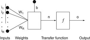
At its conceptual core, a unit in a neural network consists of three things (Figure 36.1):

1. A set of inputs that can vary in magnitude and sign coming from the outside world or from other neurons in the network.

2. A set of weights operating on these inputs that can vary in magnitude and sign (implementing synaptic efficiency and type of synapse on a neuron). There is also a bias weight b that operates on an input that is fixed to a value of 1.

3. A transfer function that converts the sum of the weighted inputs or net input, n, to an output, o.

Figure 36.1 The concept of a neural network.

The output of a unit can then become the input to another unit. Individual units are typically not very functional or powerful. Neural networks derive their power from connecting up large numbers of neurons in certain configurations (typically called layers) and from learning (i.e., setting the weights of these connections).

Neural networks are extremely good at learning a particular function (such as classifying objects). There are several different ways to train a neural network, and we will become acquainted with the most common ones in this and the next chapter.

Such trained multi-layer networks are extremely powerful. It has been shown that a suitable three-layer (i.e., three layers of units) network can approximate any computable function arbitrarily well. In other words, neural networks that are properly set up can do anything that can be done computationally. This is what makes them so appealing for applied engineering problems, because the problem solver might not always be able to explicitly formulate a solution to a problem, but he might be able to create and train a neural network that can solve the problem, even if he doesn’t understand how it works. For example, a neural network could be useful to control the output of a sugar factory given known inputs.

36.2.2 Unsupervised Learning and the Hebbian Learning Rule

Despite the fact that neural networks are very far from real biological neural networks, the learning rules that have been developed to modify the connections between computing elements in neural networks nevertheless resemble the properties of synaptic plasticity in the nervous system. In this chapter, we will focus on unsupervised learning rules (in contrast to supervised or error-correcting learning rules), which turn out to be very similar to Hebbian plasticity rules that have been discovered in the nervous system. Unsupervised learning tries to capture the statistical structure of patterned inputs to the network without an explicit teaching signal. As will be clear in a moment, these learning rules are sensitive to correlations between components of patterned inputs; they strengthen connections between components that are correlated, and weaken connections that are uncorrelated. These learning rules serve at least three computational functions: 1) to form associations between two sets of patterns; 2) to group patterned inputs that are similar into particular categories; and 3) to form content-addressable memories such that partial patterns that are fed to the network can be completed.

Donald Hebb was one of the first to propose that the substrate for learning in the nervous system was synaptic plasticity. In his book The Organization of Behavior, Hebb stated, “When an axon of cell A is near enough to excite a cell B and repeatedly or persistently takes part in firing it, some growth process or metabolic change takes place in one or both cells such that A’s efficiency, as one of the cells firing B, is increased” (1949, p. 62). In fact, William James, the father of American psychology, formulated the same idea almost sixty years earlier in his book The Principles of Psychology when he stated, “When two elementary brain-processes have been active together or in immediate succession, one of the them tends to propagate its excitement into the other” (1890, p. 566). Nevertheless, the concept of synaptic plasticity between two neurons that are co-active is usually attributed to Donald Hebb. Mathematically, Hebbian plasticity can be described as:

(36.1)

where denotes the change in synaptic weight between a presynaptic neuron i and a postsynaptic neuron j, pre_i and post_j are the activities of presynaptic neuron i and postsynaptic neuron j, respectively, and ε is a learning constant that determines the rate of plasticity. The Hebbian learning rule states that a synapse will be strengthened when the presynaptic and postsynaptic neuron are active. Neurophysiologically, this means that the synapse will be potentiated when the presynaptic neuron is firing and the postsynaptic neuron is depolarized. In 1973, Bliss and Lomo first showed that the synapses between the perforant pathway and the granule cells in the dentate gyrus of the hippocampus could be artificially potentiated using a stimulation protocol that followed the Hebbian learning rule (Bliss and Lomo, 1973). The effects of the stimulation protocol they used has been termed Long-Term Potentiation because the synapses appear to be potentiated indefinitely. Since that time, may other experiments have shown that Long-Term Potentiation could be implemented in many parts of the brain, including the neocortex. Long-Term Potentiation (with initial capital letters), which refers to an artificial stimulation protocol, should be distinguished from long-term potentiation (all lowercase), which refers to the concept that synapses may be potentiated naturally when some form of associative learning takes place.

From a computational perspective, the simple Hebbian rule can be used to form associations between two sets of activation patterns (Anderson et al., 1977). Imagine a feedforward network consisting of an input (presynaptic) and output (postsynaptic) set of neurons, f and g respectively, that are fully connected as shown in Figure 36.2. The transfer function of the f neurons is assumed to be linear and, thus, this network is referred to as a linear associator (Anderson et al., 1977). The activation of each set of neurons can be viewed as column vectors, and . Assume we want to associate a green traffic light with “go,” a red traffic light with “stop,” and a yellow traffic light with “slow.” Furthermore, assume that the green, red, and yellow traffic lights are coded as mutually orthogonal and normal (i.e., unit length) vectors.

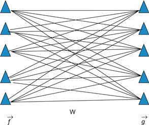
Figure 36.2 A simple linear associator network composed of an input and output set of neurons that are fully connected.

The Hebbian learning rule can be used to form these associations. Mathematically, the learning rule generates a weight matrix as an outer-product between the f and g vectors:

Now, if we probe the network with the green presynaptic pattern, we get the following:

Given that the input patterns are orthogonal to each other and normal, the output of the network is “go”:

36.2.3 Competitive Learning and Long-Term Depression

Despite its elegant simplicity, the Hebbian learning rule as formulated in Equation 36.1 is problematic because it only allows for potentiation, which means that the synapse will only grow stronger and eventually saturate. Neurophysiologically, it is known that synapses can also depress using a slightly different stimulation protocol. Fortunately, there is a neural network learning rule that can either potentiate or depress. It was proposed by Rumelhart and Zipser (1985) and is referred to as the competitive learning rule:

(36.2)

The first term on the right-hand side of Equation 36.2 is exactly the Hebbian learning rule. The second term, however, will depress the synapse when the postsynaptic neuron is active regardless of the state of the presynaptic neuron. Therefore, if the presynaptic neuron is not active, the first term goes to zero and the synapse will depress. Also, notice that depression is proportional to the magnitude of the synaptic weight. This means that if the weight is very large (and positive), depression will be stronger. Conversely, if the weight is small, depression will be weaker. The competitive learning rule can be described equivalently as follows:

(36.3)

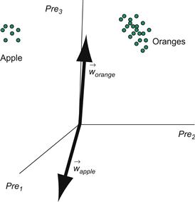
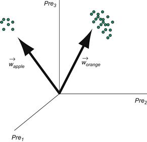
The formulation in Equation 36.3 makes clear what the learning rule is trying to do. Learning will equilibrate (i.e., terminate) when the synaptic weight matches the activity of the presynaptic neuron. On a global scale, what this means is that the learning rule is trying to develop a matched filter to the input, and can be used to group or categorize inputs. To make this clearer, consider two kinds of patterned inputs corresponding to apples and oranges. Each example of an apple or orange is described by a vector of three numbers that describe features of the object such as its color, shape, and size. Consider the problem of developing a neural network to categorize the apples and oranges (Figure 36.3).

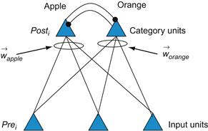
Figure 36.3 A two-layer neural network that takes input vectors corresponding to apples and oranges, and categorizes them by activating one of the two category units.

Imagine the apple and orange vectors clustered in a three-dimensional space. The weights feeding into either the apple unit or orange unit can also be viewed as vectors with the same dimensionality as the input vectors. Before learning, the apple and orange weight vectors are pointing in random directions (Figure 36.4). However, after learning, the weight vectors will be pointing toward the center of the apple and orange input vector clusters because the competitive learning rule will try to move the weight vectors to match the inputs (Figure 36.5). Finally, notice how the two category units are mutually inhibiting each other (the black circles indicate fixed inhibitory synapses which do not undergo plasticity). This mutual inhibition allows only one unit to be active at a time, so that only one weight vector is adjusted for a given input vector.

Figure 36.4 The weight vectors in an untrained competitive learning neural network.

Figure 36.5 The weight vectors in a competitive learning neural network that has been trained.

36.2.4 Neural Network Architectures: Feedforward vs. Recurrent

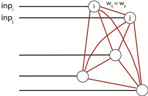
As with real neural circuits in the brain, artificial neural network architectures are often described as being feedforward or recurrent. Feedforward neural networks process signals in a one-way direction and have no inherent temporal dynamics. Thus, they are often described as being static. In contrast, recurrent networks have loops and can be viewed as a dynamic system whose state traverses a state space and possesses stable and unstable equilibria. The linear associator described above is an example of a feedforward network. The competitive learning network is a sort of hybrid network because it has a feedforward component leading from the inputs to the outputs. However, the output neurons are mutually connected and, thus, are recurrently connected. An example of a purely recurrent neural network is the Hopfield network (Figure 36.6). A Hopfield network uses a Hebbian-like learning rule to generate stable equilibria corresponding to patterns that need to be stored. By providing partial patterns of stored patterns to a Hopfield network, the network’s state will tend to progress toward its stable equilibrium corresponding to the stored pattern, and, thus, complete the pattern. This is an example of a content-addressable memory. The Hopfield network is a fully interconnected network with the constraint that connections between pairs of neurons are symmetric. Also, there are no self-connections. These constraints result in a symmetric weight matrix with zeros along the main diagonal.

Figure 36.6 The architecture of a Hopfield neural network. The weights (i.e., connections) between neurons i and j are symmetric.

36.3 Exercises

36.3.1 Competitive Learning Network

Suppose you want to categorize the following 6 two-dimensional vectors into two classes:

>> inp = [0.1 0.8 0.1 0.9 0.2 0.7;0.7 0.9 0.8 0.8 0.75 0.9];

Each column of this matrix represents one two-dimensional input vector.

There are three vectors near the (0,1) and three vectors near (1,1). What now?

First, create a two-layer network with two input “feature” neurons and two output “category” neurons. To do this, create a random 2×2 matrix of weights:

>> W=rand(NCAT,NFEATURES);

where NCAT=2 and NFEATURES=2.

Competitive learning works optimally if the weight vector associated with each output neuron is normalized to 1:

>> W=W./repmat(sqrt(sum(W.^2,2)),1,NFEATURES);

This network needs to be trained to classify properly. In this network, the output neurons compete to respond to the input in a winner-take-all fashion such that only the weight vector feeding into the winning output neuron is trained. We could implement this by including inhibitory connections between the two output neurons, and let the dynamics of the network find the winner as in Figure 36.3. To make things easier, however, we will use the max function in MATLAB® to find the winner, and then apply the competitive learning rule to the winner’s weight vector. We will also assume that the winner’s activation equals 1. Create a function that implements the competitive learning training rule with a learning rate parameter lr:

>> function [Wout]=train_cl(W,inp,lr)

>> %competitive learning rule

>> out=W*inp;

>> [mx ind]=max(out);

>> W(ind,:)=W(ind,:)+lr*(inp’-W(ind,:));

>> Wout=W./repmat(sqrt(sum(W.^2,2)),1,size(W,2));

end

Notice that the weight vectors associated with the winning output neuron are renormalized after training.

Using this training rule, create a script to classify the six input vectors. In this script, you will expose the network to all inputs one at a time over many epochs. In the script, plot the inputs and the two weight vectors (with the quiver function) associated with each output neuron after each epoch so that the learning process can be visualized (Figure 36.7).

Figure 36.7 The evolution of the two weight vectors (blue and red arrows) associated with the two output neurons during training of a competitive learning neural network. The six two-dimensional inputs are plotted as blue stars.

The results of the trained network should be:

>> results = 1 2 1 2 1 2

This indicates that the 1st, 3rd, and 5th input vectors activated neuron 1, and the 2nd, 4th, and 6th input vectors activated neuron 2. Of course, because this is an unsupervised neural network, the results could also be the exact opposite:

>> results = 2 1 2 1 2 1

You may notice that your neural network does not always categorize your inputs into two categories, but sometimes categorizes them instead into one category. This is because one of the weight vectors is accidently very far away from any input and, therefore, never wins the competition. These are called “dead units.” You will also notice that the winning weight vector is pointing in between the two classes of inputs. Can you think of a way to solve this problem?

36.3.2 Hopfield Network

We will now build a Hopfield neural network to store two four-dimensional patterns. The two column vectors we will store are:

[1 1 −1 −1]’ and [ −1 −1 1 1]’

Place those two input vectors into a 4×2 matrix called inp (i.e., the external input to the network). Create a matrix W that stores these two patterns using a Hebbian-type learning rule:

>> for ii=1:size(inp,2)

>> W=W+inp(:,ii)*inp(:,ii)’;

>> end;

>> W=W-diag(diag(W));

The last line of this code ensures that the diagonals of the weight matrix are zero. This is because the Hopfield network requires that there be no self-connectivity. Now, test to see whether those two patterns were stored in the network. To do this, write code that updates each neuron of the network with a certain probability p, which implies that not all neurons will be necessarily updated at the same time (i.e., asynchronous updating). If the neuron is updated, then a simple thresholding operation is performed. If the net input to the neuron is greater than or equal to zero, then the output of the neuron should be set to 1. Otherwise, the output of the neuron should be set to −1.

Create a function called update_hp that takes the net input, the weight matrix W, the current state of the system, and the update probability p, and updates the state of the network.

Let us now feed the trained Hopfield network with one of the two column vectors that we used to build the network: [1 1 -1 -1]′. Let us set the state of the network at t=0 to be all zeros: state(0)=[0 0 0 0]′. The net input at each time point, t, is:

>> net_input=[1 1 1 -1]’+W*state;

Therefore, at t=0, net_input(0)=[1 1 -1 -1]′. Using the net input, update the state of the network:

>> newstate=update_hp(W, state, net_input, p);

Repeat this multiple times (e.g., 1000 times) until the state of the system equilibrates.

Now feed partial input test patterns, Test, and see where the network equilibrates:

>> Test=[1 1 0 0; 0 0 −1 −1]’;

The zeros correspond to missing features in the test patterns. Does the network fill in the missing information?

36.3.3 The MATLAB Neural Network Toolbox

MathWorks has developed a specialized toolbox for neural networks. As we have shown previously, everything that constitutes a neural network (inputs, weights, transfer function, and outputs) can be implemented using matrices and matrix operations. However, the Neural Network Toolbox has a rich variety of different types of neural networks that can be easily implemented and have been optimized.

36.4 Project

Greebles live in dangerous times (Gauthier and Tarr, 1997). Recent events led to the creation of the “Department for Greeble Security.” You are a programmer for this recently established ministry, and your job is to write software that distinguishes the “good” Greebles from the “bad” Greebles (Figure 36.8). Researchers in another section of the department have shown that three parameters correlate with the tendency that a Greeble is good or bad. These parameters, identified in Figure 36.9, are: “boges” length, “quiff” width, and “dunth” height (Gauthier, Behrmann, and Tarr, 2004). Specifically, it has been shown that good Greebles have long boges, thin quiffs, and high dunths, while the bad Greebles tend to have short boges, thick quiffs, and low dunths. Of course, this relationship is far from perfect.

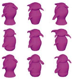
Figure 36.8 Meet the Greebles. Image courtesy of Michael J. Tarr, Brown University, http://www.tarrlab.org/.

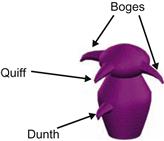
Figure 36.9 The anatomy of a Greeble. Image courtesy of Michael J. Tarr, Brown University, http://www.tarrlab.org/.

A given individual Greeble might have any number of variations of these parameters. In other words, this classification is not as clear-cut and easy as your superiors might want it to be. That’s where you come in. You decide to solve this problem with a neural network, since you know that neural networks are well-suited for this kind of problem.