3

Structure of Measuring Systems

The aspects for valid measurement are the transducer, the structure, and system dynamics, as shown in Fig. 1-7. The transducer and process of sensing were examined in Chapter 2. In this chapter we present the structural aspect or the arrangement of components in a measuring system. Topics included are methods of measurement, interaction between components, transducer circuits. System dynamics are examined in Chapter 4.

3-1.  METHODS OF MEASUREMENT

Methods of measurement are the null balance and the unbalance method. Other methods can be viewed as variations of these two. Models showing principles of instruments based on these methods are described. A comparison of the characteristics of the models is presented in the next section.

The process of sensing and methods of measurement are summarized in Table 3-1. The first two columns of the table are similar to those in Table 1-2. The first column is an open-ended list of measurands and the second is an open-ended list of phenomena or physical laws for sensing. Numerous instruments utilizing combinations of these items are commonly used, yet there are essentially only two basic methods of measurement, as shown in the third column.

A.  Null-Balance Method

The null-balance method compares the unknown value of a measurand with that of a reference standard. The system is nulled or balanced prior to a measurement. The unknown and the standard are then applied to the system. The standard is adjusted until the system is again nulled. Thus the value of the measurand is equal to that of the standard. The technique uses the effect of the standard on the system to oppose that of the measurand until there is no detectable output.

TABLE 3-1 Relation of Measurands, Sensors, and Methods of Measurement

Measurand	Phenomena for sensing	Method of measurement
Flow	Pressure drop
Temperature→	Resistance change	Null balance method
Pressure	Inductance change	Unbalance method
Motion	Capacitance change

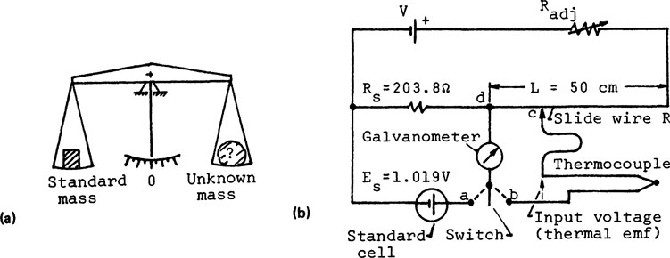
For example, the chemical balance shown in Fig. 3-1 is initially nulled before an unknown mass is applied. The mass added will upset the balance. The standard mass is introduced and adjusted to restore the balance to its original null position. Hence the value of the unknown mass is equal to that of the standard. The method essentially compares the effect of the unknown mass on the balance with that of the standard. The output of the balance is zero prior to a measurement and is also zero at the end of the measurement.

The thermocouple potentiometer for temperature measurement, shown in Fig. 3-1b, is another example. It compares the thermal EMF from a thermocouple with that of a standard voltage. The instrument consists of a working battery V in series with an adjustable resistor R_adj, a uniform slide wire of resistance R, and a precision resistor R_s. The slide wire R can be calibrated to become a variable standard voltage source.

FIGURE 3-1 Examples of null-balance instruments. (a) Chemical balance. (b) Thermocouple potentiometer.

First, the instrument is calibrated by means of a standard cell V_s. The resistor R_adj is adjusted and the galvanometer is switched momentarily to position a. The galvanometer will show no deflection if the voltage across R_s due to the battery V is equal to that of the standard cell. Thus the voltage across R_s is standardized to 1.019 V. Since R and R_s are in the same loop, the slide wire R is also calibrated. Let R = 10 Ω, R = 203.8 Ω, and the standard voltage V_s = 1.019 V. Hence the voltage across R is (1.019)(JR/R_a) = 1.019(10/203.8) = 0.05 V. If the length of the slide wire R is 50 cm, it is calibrated to 1.0 mV/cm.

Second, the EMF from the thermocouple is compared with the voltage along R. The contact c is moved along R and the galvanometer is switched momentarily to position b. When it shows no deflection upon switching to position b, the voltage from d to c along R is equal to the thermal EMF of the thermocouple. In other words, the instrument is again nulled at the end of a measurement. When the thermal EMF is equal and opposite to the voltage from d to c of the slide wire R, there is no current flow in the thermocouple circuit. Thus the measurement is independent of the resistance of the thermocouple and the length of the lead wires, and there is no energy transfer between the thermocouple circuit and the potentiometer.

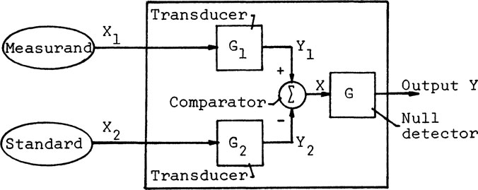
The model of a null-balance instrument is shown in Fig. 3-2. The input X₁ is the measurand and X₂ the reference standard. The transducers G₁ and G₂ are assumed identical. The outputs Y₁ and Y₂ are compared by means of a comparator or a null detector G, which is a high-gain amplifier. Any difference between the inputs X₂ and X₂ is greatly magnified.

The equations describing the system are as follows:

$\begin{array}{ll}{Y}_1=G_1{X}_1\hfill & Y_2=G_2{X}_2\hfill \end{array}$

(3-1)

$\begin{array}{ll}X=Y_1-Y_2\hfill & Y=GX\hfill \end{array}$

(3-2)

FIGURE 3-2 Models of null-balance instruments.

$Y=G\left(G_1{X}_1-G_2{X}_2\right)$

(3-3)

$Y=G\left[G_{\text{av}}\left(X_1-X_2\right)\right]$

(3-4)

where G_av = (G₁ + G₂)/2 ≃ G₁ ≃ G₂. When the instrument is nulled, the output is Y = 0, giving X₁ = X₂.

The requirements of the null-balance method are that (1) the inputs X₁ and X₂ produce the same effect on the instrument, (2) G is very sensitive near the null psoition, and (3) G is insensitive away from null. When the system is unbalanced, the requirement is that the sensitivity is sufficient only to indicate the direction for restoring the system to null.

A null-balance instrument is capable of high sensitivity and precision by having G in Eq. 3-4 very large for detecting a small difference in (X₁ – X₂). The instrument is also capable of high accuracy, because a reference standard is used for the measurement. Except for the null balancing, the instrument does not have to be calibrated for its range of operation.

Note that the accuracy of the null instrument does not imply equal accuracy for a measurement. For example, the potentiometer itself can be very accurate in comparing the EMF of a thermocouple with that of a reference voltage, but the thermocouple is external to the potentiometer. When the thermal EMF is measured precisely and accurately, it is not automatic that the temperature is also evaluated with equal precision or accuracy.

Finally, only (1) like quantities and (2) quantities of the same order of magnitude can be compared. A force is compared with another force, and a color with another color. The comparison of two unlike quantities is like comparing apples and oranges. Furthermore, the quantities being compared must be of the same order of magnitude. An old Chinese proverb says, “The water in an ocean cannot be measured with a drinking cup.” The size of an atom could not be measured until the discovery of x-rays, the wavelength of which is comparable to the dimension of atoms.

B.  Unbalance Method

For the unbalance method, the effect of the input on the instrument is manifested as an output. The input and output are generally different physical quantities, such as a mechanical input with an electrical output. Hence it is also called the analogous method.

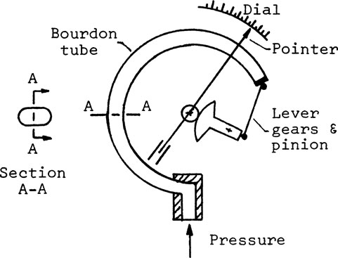
The common bourdon tube pressure gage shown in Fig. 3-3 is an example of an unbalance instrument. The bourdon tube is elliptical in cross section. The pressure forces the tube to become more circular, thereby causing a deflection at the free end of the tube. The deflection is magnified with levers and gears to rotate a pointer for a dial reading. Thus the input is pressure and the output is an angular deflection of the pointer analogous to the input pressure.

FIGURE 3-3 Bourdon tube pressure gage.

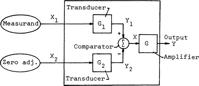
The model of an unbalance instrument shown in Fig. 3-4 is similar to that shown in Fig. 3-2 for the null-balance instrument, except that a zero adjustment is substituted for the reference input. The instrument is initially adjusted to zero. For example, the levers and gears of the pressure gage in Fig. 3-3 are initially adjusted to indicate zero gage pressure. The initial conditions of an unbalance instrument are

$Y=G\left(G_1{X}_{10}-G_2{X}_{20}\right)=0$

where X₁₀ is due to some internal unbalance in the instrument and X₂₀ is the initial zero adjustment. When the measurand X₁ is applied, we get

$\begin{array}{lll}Y\hfill & =\hfill & G\left[G_1\left(X_1+X_{10}\right)-G_2{X}_{20}\right]\hfill \\ Y\hfill & =\hfill & G{G}_1{X}_1\hfill \end{array}$

(3-5)

Terminology for methods of measurement is not standardized. While not intending to “set the record straight,” let us comment briefly on the topic. An unbalance method only implies that the input is not balanced by means of a reference standard. Internally, all systems must be in equilibrium, such that the static and dynamic forces must balance. The unbalance method is variously called indirect, deflection, or analogous. The term indirect stems from the fact that the null balance method is called the direct (comparison) method. Since all measurements are based on physical laws, it is difficult to say that one law is more direct than another. The term deflection implies a dial reading, while some instruments are digital. The output of a null balance or an unbalance instrument can be analogous to the input. The terms null balance and unbalance seem sufficiently descriptive for this book.

FIGURE 3-4 Model of unbalance instruments.

C.  Differential Method

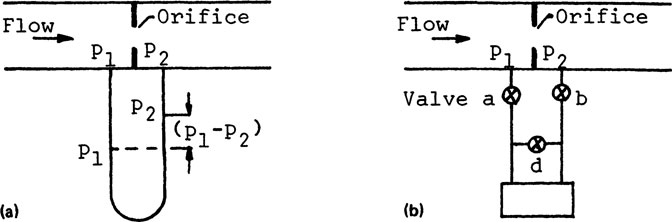
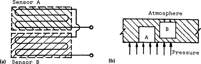
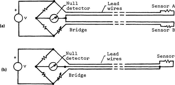
A differential measures the difference of two like quantities. Every car has a differential. A differential manometer for a flow measurement is shown in Fig. 3-5a. For remote sensing, an electrical differential pressure transducer is substituted, as shown in Fig. 3-5b.

The differential method is a variation of the null-balance method. The instrument is nulled prior to a measurement. The inputs X₁ and X₂ are applied, as shown in the model in Fig. 3-2, but X₂ is a second input and not a reference standard. Only the difference (X₁ – X₂) is of interest. From Eq. 3-3 we get

$Y=G\left[G_{\text{av}}\left(X_1-X_2\right)\right]$

(3-6)

where G_av = (G₁ + G₂)/2 ≃ G₁ ≃ G₂. When G₁ and G₂ are not identical, it can be shown by simple algebra that

$\underset{\text{output}}{\underbrace{Y}}=\underset{\text{signal}}{\underbrace{G[G_{\text{av}}\left(X_1-X_2\right)}}+\underset{\text{noise}}{\underbrace{\left(G_1-G_2\right)X_{\text{av}}]}}$

(3-7)

where X_av = (X₁ + X₂)/2 is called the common mode. The signal and the noise terms are identified in Eq. 3-7. When G₁ is not identical to G₂, a noise component is always present in a differential measurement.

FIGURE 3-5 Differential devices for flow measurement. (a) Differential manometer. (b) Differential pressure transducer.

A rearrangement of Eq. 3-7 gives the signal/noise ratio.

$Y=G\left[G_{\text{av}}\left(X_1-X_2\right)\right]\left[1+\frac{\left(G_1-G_2\right)X_{\text{av}}}{G_{\text{av}}\left(X_1-X_2\right)}\right]$

(3-8)

$Y=\underset{\text{desired signal}}{\underbrace{\left(G{G}_{\text{av}}\right)\left(X_1-X_2\right)}}\left(1+\frac{\text{noise}}{\text{signal}}\right)$

(3-9)

G_av/(G₁ – G₂) is the common-mode-rejection ratio [1]. It is a part of the specification and a figure of merit indicating the ability of an instrument to reject the common mode. G_av is the gain or amplification of the signal (X₁ – X₂). (G₁ – G₂) is the gain of the common mode X_av. The gain of the signal is compared with that of the common mode in Eq. 3-8. The signal/noise ratio is deduced in Eq. 3-9. In electronic instruments, the rejection ratio is dependent on the magnitude and frequency of the signal as well as the sensitivity setting of the instrument. It is intuitive that the larger the common mode, the larger the noise component in the output. In other words, when X_av is very large, the instrument attempts to take the difference between two large quantities of almost equal magnitude.

The noise output is due to an imbalance in G₁ and G₂. Consider the differential pressure transducer shown in Fig. 3-5b as an example. Assume that G₁ = 101, G₂ = 99, and X_av/(X₁ – X₂) = 15/1. From Eq. 3-8 we obtain

$\begin{array}{lll}Y\hfill & =\hfill & G\left(100\right)\left(X_1-X_2\right)\left(1+\frac{101-99}{100}\frac{15}{1}\right)\hfill \\ \hfill & =\hfill & G\left(100\right)\left(X_1-X_2\right)\left(1+0.30\right)\hfill \end{array}$

The example shows that when G₁ and G₂ differ by ±1% and the average pressure to the differential pressure has a ratio of 15:1, the noise can be as high as 30% of the signal.

The noise due to the common mode can be evaluated by applying identical inputs to a differential instrument. For the differential pressure transducer in Fig. 3-5b, the pressure inputs can be equalized by closing valve b and opening valve d. Thus, any output is a noise due to the common mode.

D.  Inferential and Comparative Measurements

An inferential measurement is one in which the value of a measurand is calculated or inferred from the measurement of other physical quantities. The method is used when a more direct measurement is less convenient or when a transducer cannot be placed at the desired location. Inferential also implies the measurement of quantities other than the measurand.

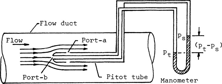
For example, the measurement of air velocity by means of a pitot tube shown in Fig. 3-6 is inferential. The pitot tube consists of an inner and an outer tube separated by an annular space. The assembly is aligned with the direction of flow. Port a of the outer tube is normal to the flow and it measures only the static pressure p_s. Let p_υ be the pressure due to the velocity υ. Port b of the inner tube points upstream. It measures the total pressure p_t, which is the sum of p_s and p_υ:

$\begin{array}{ll}{p}_t\hfill & =p_s+p_{\upsilon }\text{and}{p}_{\upsilon }=\frac{1}{2}\text{ρ}{\upsilon }^2\hfill \\ \upsilon \hfill & ={\left[\frac{2}{\text{ρ}}\left(p_t-p_s\right)\right]}^{1/2}\hfill \end{array}$

FIGURE 3-6 Pitot tube for fluid velocity measurement.

where ρ is the mass density of the fluid. The velocity υ is inferred from the pressure information.

Note that all measurements are inferential in the sense that they are inferred by means of physical laws. For a pressure gage, the pressure is inferred from the elastic deformation of the bourdon tube, according to the stress-strain relation of the material. For a resistance strain gage, the strain is inferred by means of a resistance change. For the pitot tube, flow velocity is inferred from measurements of pressure. It is true that some measurements are made more directly than others. Nonetheless, they are all inferred from physical laws.

A comparative method compares the characteristics of an object with the corresponding characteristics of another. The technique is extremely useful, but the measurement is meaningful only on all-things-equal basis. For example, the viscosity of lubricating oils is expressed in Saybolt Universal Seconds [2]. The method determines the viscosity of oil by timing the flow of a certain quantity through a short capiliary tube under specified conditions. The measurement is meaningful only for comparing two oils that are identical in every respect except for viscosity. Pushing the argument to the extreme, a comparison of the viscosity of lubricating oil with that of syrup is meaningless.

Comparative tests are often the bases for specifications and acceptance tests in industries [3]. Executing the tests under standardized conditions is relatively straightforward. Interpretation of the test results is vastly more difficult. For a machine tool, the results from laboratory tests at one cutting speed must not be used for predicting the performance at speeds used in practice. Ideally, a performance test should give information about the behavior of the machine tool for all possible cutting operations [4]. The ultimate performance of a machine must depend on its inherent quality and conditions of application. A comparative test is meaningful only on an all-things-equal basis. This reemphasizes the discussion in Chapter 2 that a static calibration cannot be extrapolated automatically for dynamic applications.

3-2.  COMPARISON OF METHODS OF MEASUREMENT

The null-balance and unbalance methods represent two principles of measurement. Their characteristics are examined in this section.

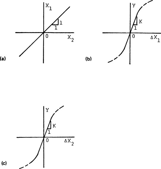
For a null-balance instrument, the measurand X₁ is linear with the reference standard X₂, as shown in Fig. 3-7a. Note that as long as the system can be balanced before and after a measurement, the null balance instrument itself can be nonlinear. The instrument is balanced when X₁ = X₂, and the output is

FIGURE 3-7 Characteristics of null-balance systems. Model shown in Fig. 3-2. (a) X₁ versus X₂. (b) Y versus ΔX₁ (c) Y versus ΔX₂.

$\begin{array}{lll}Y=f_1\left(X_1-X_2\right)=0\hfill & \text{for}\hfill & X_1-X_2\hfill \end{array}$

(3-10)

A small unbalance exists when

$\begin{array}{lll}Y=f_2\left(\Delta X\right)\ne 0\hfill & \text{for}\hfill & \left(X_1-X_2\right)=\Delta X\hfill \end{array}$

(3-11)

The instrument is made very sensitive for any unbalance ΔX, whether X₁ is larger or smaller than X₂ as shown in Fig. 3-7b and Fig. 3-7c. The sensitivity is the slope K shown in Fig. 3-7b. K can be large about null when the instrument is almost balanced. For a large unbalance, however, only the direction of the deviation from null is needed for restoring the instrument to its high-sensitivity region. It is neither practical nor necessary to maintain a very high sensitivity over a wide range. Since the sensitivity of a null balance instrument is not constant, the null detector is inherently nonlinear.

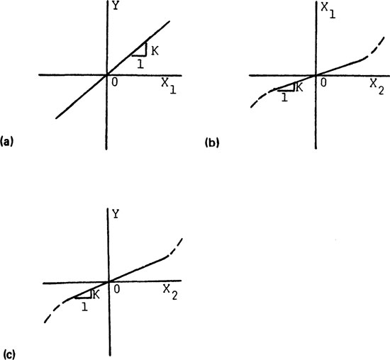
For an unbalance instrument, the sensitivity K relating the output Y and the input X₁ is constant for its entire linear range, as shown in Fig. 3-8a. K cannot be excessive in order to maintain a reasonable scale at the output. At the same time, the instrument should be fairly insensitive to the initial zero adjustment X₂. Hence both the input X₁ and the output Y are insensitive to X₂, as shown in Fig. 3-8b and Fig. 3-8c.

Advantages of the null-balance systems are high sensitivity and high accuracy, and minimal loading due to energy transfer.

1.  High sensitivity is possible because the instrument measures only small deviations about a null point, as shown in Fig. 3-7b and Fig. 3-7c. The potential for high accuracy is by virtue of the high sensitivity and the comparison with a reference standard. An example of the null-balance instrument with high accuracy is a servo-accelerometer [5]. It has a built-in servomechanism to balance the internal forces within the accelerometer. By comparison, a piezoelectric accelerometer [6] is an unbalance transducer and is less accurate.

FIGURE 3-8 Characteristics of unbalance systems. Model shown in Fig. 3-4. (a) Y versus X₁ (X₂ constant). (b) X₁ versus X₂. (c) Y versus X₂ (X₁ constant).

2.  Loading due to energy transfer in a null balance instrument is minimal. For the thermocouple potentiometer shown in Fig. 3-1b, there is no current flow in the thermocouple circuit at null. Thus there is no energy exchange between the thermocouple and the potentiometer.

Disadvantages of the null-balance systems are the added complexity and cost, and the additional time required for balancing the instrument.

1.  The additional complexity is self-evident. As Henry Ford once said: “The gadgets you left off the car cannot cause you trouble.”

2.  A null balance instrument is inherently slower than an unbalance instrument. It takes time for the balancing, even when it is done automatically. For example, the frequency range of a servo-accelerometer is much lower than that of a piezoelectric type.

Unbalance instruments are generally faster in response and less expensive. They are more commonly used for dynamic measurements. An unbalance system must be calibrated for its operating range, since the measurement is not compared with a standard.

Due to the differences in performance characteristics shown in Figs. 3-7 and Figs. 3-8, an instrument designed for the null balance method will not be suited for the unbalance method, and vice versa. A comparison of the performance of the two types of instruments is given in an excellent paper by Stein [7].

3-3.  INTERACTION BETWEEN COMPONENTS

Components are interconnected to form a measuring system. The interaction between components is examined in this section by means of input/output impedances. The types of components considered at the one-, two-, and three-port devices.

A.  Concept of Impedance

Impedance is that which impedes a flow. For electrical systems, a flow is the current through a component. For mechanical systems, impedance is defined from the generalization of Ohm’s law, but the definitions are not standardized [8]. Using the force-voltage analogy, the “flow” in a mechanical system is velocity. Analogies will be used for the discussions to follow, but generalized impedance, the classification of types of energies, and related topics are not presented.

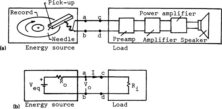
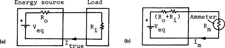
Let us use examples to illustrate the concept of input/output impedance. The schematic of a hi-fi phono system is shown in Fig. 3-9a. In formation is transferred from the energy source to the load. The energy source includes all components upstream of the interface at terminals a and b, including the turntable, the phono record, the needle, and the pickup. Certain quantities, such as the speed of the turntable and the ac power supply, are constants. They are omitted from considerations in dynamic analysis. The energy source is modeled by means of its Théve nin’s equivalent, consisting of an equivalent voltage source V_eq in series with an output impedance R_o, as shown in Fig. 3-9b. The load includes all components downstream from terminals c and d. Since the load does not have an energy source, it is modeled by means of an input impedance R_i as shown in Fig. 3-9b.

FIGURE 3-9 Example of input/output impedance. (a) Schematic of a hi-fi system. (b) Thévenin’s equivalent.

The representation in Fig. 3-9b is a general model, from which the interaction between an energy source and load is derived. At an interface dividing a measuring system, the components can be grouped as up-stream and downstream from the interface, and their interaction studied by means of this model.

The output impedance R_o limits the power than an energy source can deliver. Let an energy source, such as a D-cell, be represented by its Thevenin’s equivalent, as shown in Fig. 3-9b. The D-cell is connected to a resistor R_i. The loop equation is

$V_{\text{eq}}=\left(R_o+R_i\right)I$

(3-12)

where V_eq is an ideal voltage source, R_o the output impedance of the source R_i the input impedance of the load, and I the loop current. Since and R_o are constant, I increases as R_i decreases. If R_o = 0 and R_i approaches zero, the current I would become infinite. It would be possible to get an infinite current from the D-cell. This is not possible because R_o must exist and it is the internal to the energy source. It limits the current that the D-cell can deliver.

Returning to the phono recorder player in Fig. 3-9a, the pickup is an energy source and it delivers “power” downstream. Since its power is derived entirely from the movement of the needle, its capacity for power delivery must be small. Hence the output impedance R_o of the pickup must be high in order to limit the power delivery. If R_o were low, it would be possible to drive the speakers directly from the phono pickup.

The input impedance R_i determines the capacity of a load to absorb power. From Fig. 3-9b the power P delivered to the load is

$P=I^2{R}_i=\frac{V_o^2}{R_i}$

(3-13)

where V_o is the actual voltage across R_i. A large value of R_i is necessary to minimize the energy (power) transfer between the energy source and the load. In practice, a phono pickup is connected to a preamplifier (preamp), which has an extremely high input impedance. This minimizes the loading of the pickup. Furthermore, the preamp has a low output impedance in order to deliver sufficient power to the components downstream.

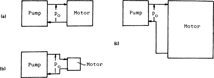
To further elaborate on the concept of impedance, consider the hydraulic pump-and-motor assembly shown in Fig. 3-10a. The pump is properly sized for the motor. A worker uses the same pump to drive a smaller motor, as shown in Fig. 3-10b, and the setup works satisfactorily. To meet a higher power demand, the worker connects the same pump to a much larger hydraulic motor, as shown in Fig. 3-10c. The engineer refuses to authorize the setup, on the ground of impedance mismatch. Although the pump and the motors have the same pressure rating, it takes pressure and flow to deliver power.

The hydraulic pump-and-motor assembly can be modeled in Fig. 3-9b. Assume that the pump is represented by its Thévenin’s equivalent, with a V_eq and R_o in series. The motor is represented by an input impedance R_i. A small hydraulic motor has small passages and therefore a high input impedance R_i. A large motor has large passages and therefore low input impedance. The loop equation for the assembly is

$V_{\text{eq}}=\left(R_o+R_i\right)I$

FIGURE 3-10 Hydraulic pump and motor. (a) Pump and hydraulic motor—properly sized. (b) Pump with small motor. (c) Pump with large motor.

When the pump drives the small motor, R_o ≪ R_ι of the motor. The loop equation becomes

$\begin{array}{lll}{V}_{\text{eq}}=R_{i}I\hfill & \text{for}\hfill & R_o\ll R_{\iota }\hfill \end{array}$

(3-14)

The pump appears as an ideal potential source, since V_eq is constant and the flow I depends on R_i of the motor. In other words, the small motor is driven at its rated pressure, and the flow depends on the size of the motor.

When the same pump drives a much larger motor, R_o ≫ R_ι of the motor. The loop equation becomes

$\begin{array}{lll}{V}_{\text{eq}}=R_{o}I\hfill & \text{for}\hfill & R_o\gg R_{\iota }\hfill \end{array}$

(3-15)

Since V_eq and R_o are constant, the flow I is constant. The pump becomes a constant delivery pump, or an ideal flow source. Note that the internal V_eq, does not changed, but the supplied pressure V₀ at the inlet of the motor cannot be maintained by the pump.

In summary, the output impedance R_o of a power source limits its ability to delivery power at a given potential level, and the input impedance R_i of a load determines its capacity for power absorption, as shown in Eq. 3-13. A power source becomes a constant potential source when R_o ≪ R_i, and a constant flow source when R_o ≫ R_i.

Impedance matching describes conditions for minimum loading due to power transfer, or maximum power transfer between adjacent components. Minimum loading is examined in the next section. Maximum power transfer is desired only at the output power stage of instruments. The power P delivered is

$P=I^2{R}_i$

Substituting I = V_eq/(R_o + R_ι) from Eq. 3-12 gives

$P={\left(\frac{V_{\text{eq}}}{R_o+R_{\iota }}\right)}^2{R}_{\iota }$

Differentiating the equation with respect to R_o and equating the derivative to zero for maximum, we get

$\begin{array}{ll}{R}_o=R_{\iota }\hfill & \text{for maximum power transfer}\hfill \end{array}$

(3-16)

B.  One-Port Devices

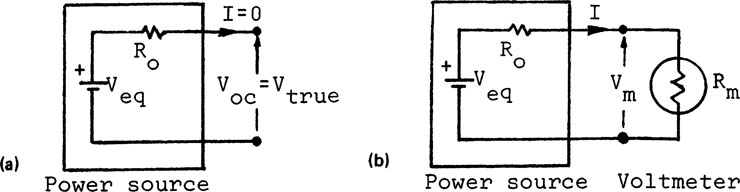
A one-port device has one port for energy transfer. The device is either an energy source or a load, as shown in the model in Fig. 3-9b. The energy source is the source of information and is represented by its Thévenin’s equivalent. The load is a transducer or a meter for the measurement. The energy transfer between the source and the load will cause a loading. Loading, such as in a voltage measurement, will be described in this section.

Consider a voltage or a potential measurement The true voltage V_true, is the open-circuit voltage before the meter is connected, as shown in Fig. 3-11a. Since I = 0, V_oc = V_true = V_eq. A voltmeter of input impedance R_m for the measurement is shown in Fig. 3-11b. R_m and R_o form a voltage divider for V_eq and the measured voltage V_m is

$\begin{array}{lll}\frac{V_m}{V_{\text{eq}}}=\frac{R_m}{R_m+R_o}\hfill & \text{or}\hfill & V_m\hfill \end{array}=\frac{1}{1+R_o/R_m}{V}_{\text{true}}$

(3-17)

The measured voltage is always less than the true voltage. V_m approaches V_true when R_m ≫ R_o. Hence a voltmeter should have a high input impedance. A rule of thumb is that R_m/R_o > 10:1.

This conclusion can be deduced directly from the discussions on energy models in Sec. 2-3B. For a voltage measurement, the current is secondary. Hence R_m of the voltmeter must be very high in order to limit the current flow for minimal loading.

FIGURE 3-11 Voltage measurement. (a) Before. (b) After.

The model study is not restricted to electrical systems. For electrical measurements, a voltmeter with extremely high input impedance is readily available, and loading due to energy transfer is usually not a problem. For a complex problem, such as in bioengineering [9], the output impedance of the source of information and the input impedance of the primary sensor must be well considered.

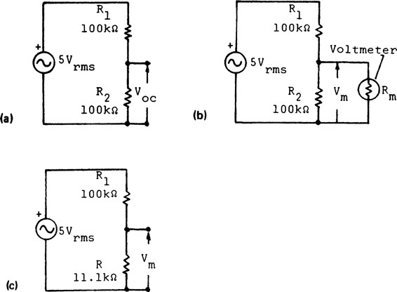
Example 3-1. Find the measured voltage V_m in Fig. 3-12a. Assume that the input impedance of the voltmeter is 5 kΩ/V_ac.

Solution: Since an output of 2.5 V is anticipated, the meter is set at the range 0 to 2.5 V. Thus R_m of the meter is

$R_m=\left(5\text{k}\Omega /{\text{V}}_{\text{ac}}\right)\left(2.5\text{V}\right)=12.5\text{k}\Omega$

The equivalent resistance, due to R_m and R₂ in parallel in Fig. 3-12b is R = (12.5)(100)/(12.5 + 100) = 11.1 kΩ. R and R₁ form a voltage divider for V_eq in Fig. 3-12c. The measured voltage is

$V_m=\frac{R}{R+R_1}\times 5\text{V=}\frac{11.1}{11.1+100}\times 5\text{V=0}\text{.5}\text{V}$

FIGURE 3-12 Loading in voltage measurement. (a) Before. (b) After. (c) Equivalent.

Note that V_m = 0.5 V is less than the 2.5 V anticipated. It can be demonstrated that this is the actual measured voltage.

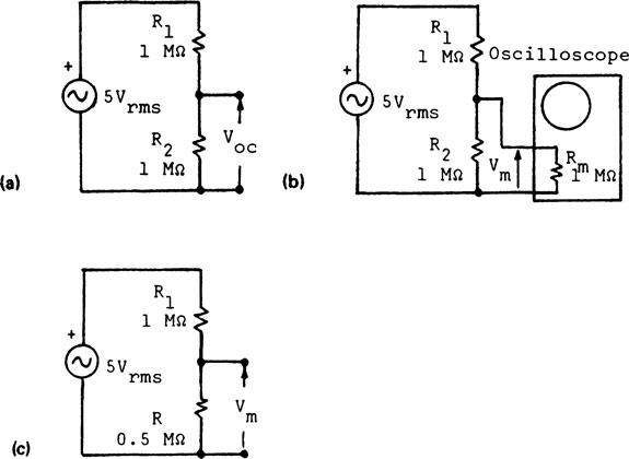
Example 3-2. Find the peak-to-peak voltage V_p-p indicated by the oscilloscope in Fig. 3-13a. Assume that the input impedance R_m of the oscilloscope is 1 MΩ and its sensitivity is at 1 V/cm.

Solution: The anticipated measured voltage is 2.5 V_rms or $2\times 2.5\sqrt{2}=7.07V_{\text{p}-\text{p}}.$ The equivalent resistance, due to R_m and R₂ in parallel in Fig. 3-13b, is 0.5 MΩ. From the equivalent circuit in Fig. 3-13c, the measured voltage V_m is

$V_m=\frac{R}{R+R_1}\times 5{\text{V}}_{\text{rms}}=\frac{0.5\times 5}{0.5+1}=1.67{\text{V}}_{\text{rms}}$

The observed peak-to-peak voltage is $V_{\text{p}-\text{p}}=2\times 1.67\sqrt{2}=4.71\text{V or 4}\text{.7cm,}$ but the anticipated V_p-p is 7.1 V or 7.1 cm. An expensive oscilloscope can have a large error of 33% in a simple voltage measurement.

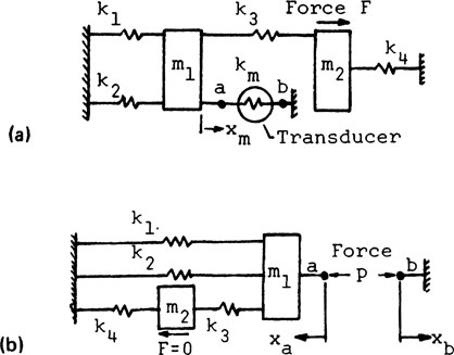
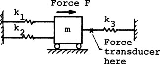
Example 3-3. A force F is applied to a system shown in Fig. 3-14a, where the k’s are the stiffness of the springs. A force transducer of stiffness k_m, shown in Fig. 3-14b, is inserted to measure the static force transmitted through k₂. Find the error in the force measurement by means of Thévenin’s theorem using the force-voltage analogy. (The problem can be solved directly instead of using Thévenin’s theorem, as shown in Fig. 3-14c.)

FIGURE 3-13 Loading in voltage measurement. (a) Before. (b) After. (c) Equivalent.

FIGURE 3-14 Loading in static force measurement. (a) Before. (b) After. (c) Direct calculation. (d) Thévenin’s theorem.

Solution: The ratio F_m/F_true is deduced directly from Eq. 3-17 by analogy, where F_m is analogous to V_m, k_m to R_m, and k_o to R_o.

$F_m=\frac{1}{1+k_o/k_m}{F}_{\text{true}}$

(3-18)

The output stiffness k_o is determined by applying a force p at the interface at terminals a and b of the force transducer and noting the corresponding deflections, as shown in Fig. 3-14d. Note that F = 0 in applying Thévenin’s theorem. The method is analogous to using Ohm’s law for finding the resistance of a network by applying a voltage V and noting the current I. Thus

$k_o=\frac{\text{force}}{\text{deflection}}=\frac{p}{x_a+x_b}$

(3-19)

$k_o=\frac{P}{P/k_2+P/\left(k_1+k_3\right)}=\frac{k_2\left(k_1+k_3\right)}{k_1+k_2+k_3}$

(3-20)

Substituting k_o from Eq. 3-20 into Eq. 3-18, we get

$\frac{F_m}{F_{\text{true}}}=\frac{k_m\left(k_1+k_2+k_3\right)}{\left(k_1+k_3\right)\left(k_2+k_m\right)+k_2{k}_m}$

The corresponding fraction error is

$\frac{F_m}{F_{\text{true}}}=\frac{k_m\left(k_1+k_2+k_3\right)}{\left(k_1+k_3\right)\left(k_2+k_m\right)+k_2{k}_m}$

Error in a flow measurement is due to the obstruction introduced by the meter in the flow circuit. The true current I_true shown in Fig. 3-15a is before an ammeter is inserted in the circuit. The measured current I_m shown in Fig. 3-15b is after the meter R_m is inserted. The loop equations from the figures are

$V_{\text{eq}}=\left(R_o+R_i\right)I_{\text{true}}$

(3-21)

$V_{\text{eq}}=\left[\left(R_o+R_{\iota }\right)+R_m\right]I_m$

(3-22)

From the equations above, we get

$I_m=\frac{1}{1+R_m/\left(R_o+R_i\right)}{I}_{\text{true}}$

(3-23)

Hence the input impedance R_m of the ammeter must be low for a true flow measurement. In other words, the voltage in a current measurement is secondary, and the voltage drop across the ammeter must be low for minimal loading.

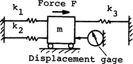
Example 3-4. A force F is applied at m₂ shown in Fig. 3-16a. The static deflection at m₁ is measured by means of a transducer of stiffness k_m. Find the ratio x_m/x_true, where x_m and x_true are the displacements at m₁ before and after the transducer is applied.

Solution: The m’s and k’s in the system are rearranged as shown in Fig. 3-16b for convenience. A force p is introduced to find the output stiffness k_o of the system. Thus

$\begin{array}{ll}{k}_o\hfill & =\frac{\text{force}}{\text{deflection}}=\frac{p}{x_a+x_b}\hfill \\ {\text{k}}_0\hfill & =\frac{p}{p/k_{\text{eq}}+0}=k_{eq}=\left(k_1+k_2\right)+\frac{k_3{k}_4}{k_3+k_4}\hfill \end{array}$

FIGURE 3-15 Current measurement. (a) Before. (b) After.

FIGURE 3-16 Loading in static displacement measurement. (a) System. (b) To find k₀.

where k_eq is due to the series-parallel combination of the k’s. By analogy from Eq. 3-23, we have

$\begin{array}{lll}{x}_m\hfill & =\hfill & \frac{1}{1+k_m/k_o}{x}_{\text{true}}\hfill \\ x_m\hfill & =\hfill & \frac{\left(k_1+k_2\right)\left(k_3+k_4\right)k_3{k}_4}{\left(k_1+k_2+k_m\right)\left(k_3+k_4\right)+k_3{k}_4}{x}_{\text{true}}\hfill \end{array}$

(3-24)

C.  Two-Port Devices

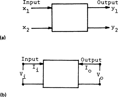
A two-port device represents an intermediate component in a measuring system. It has two ports for energy transfer, with two variables at the input port and two at the output port. In this section we discuss the parameters commonly used for describing two-port devices and illustrate their applications under static and sinusoidal steady-state conditions.

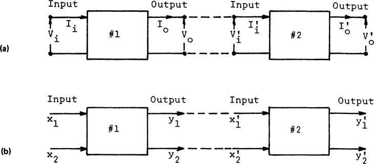
The four variables of a two-port in Fig. 3-17 are related by a set of simultaneous equations (see Eq. 2-28), such as

$\begin{array}{lll}{y}_1=f_1\left(x_1,y_2\right)\hfill & \text{and}\hfill & x_2=f_2\left(x_1,y_2\right)\hfill \end{array}$

(3-25)

where the x’s are variables at the input and the y’s at the output. Technique for deriving the parameters from the equations for the incremental model was described in Sec. 2-3C. In general, the parameters are constants for static applications and are complex numbers under sinusoidal steady-state conditions.

FIGURE 3-17 Models of two-port devices. (a) Transducer. (b) Network.

A two-port device has four variables, but only two of them can be independent. There are six combinations of four variables taken two at a time. Hence there exist six sets of simultaneous equations for describing a two-port device, one of which is shown in Eq. 3-25. The choice of equations depends on the results desired and the ease with which the parameters can be evaluated. Furthermore, these are four parameters in the incremental model for each set of the simultaneous equations as shown in Eq. 2-31. From the six combinations, there exist a total of 24 parameters for describing the same system.

The system will behave in its own way, however, regardless of the equations selected for its description. Thus the parameters from one description must be convertible to those from the others. Readers should not be confused by the large number of parameters in the literature for describing a device, such as a transistor. A familiarity with one set of parameters will lead logically to the interpretation of the others.

For convenience, voltage V and current I will be used to denote potential and flow in the discussions to follow. It is understood that the discussions are equally applicable for nonelectrical systems. The sign convention for network analysis in Fig. 3-17b will be used unless otherwise stated. The parameters commonly used for describing a two-port are presented below.

1.  Z Parameters

When the currents in Fig. 3-17b are the independent variables, the parameters are impedances or z parameters. The functional relations are

$\begin{array}{lll}{V}_i=f_1\left(I_i,I_o\right)\hfill & \text{and}\hfill & V_o=f_2\left(I_i,I_o\right)\hfill \end{array}$

(3-26)

where the subscript i denotes the input and o the output variables. Following the derivations from Eqs. 2-28, 31, we get

$\begin{array}{ll}\begin{array}{l}{V}_i=z_i{I}_i+z_r{I}_o\hfill \\ V_o=z_f{I}_i+z_o{I}_o\hfill \end{array}\hfill & \begin{array}{llll}\left[\begin{array}{l}{V}_i\hfill \\ V_o\hfill \end{array}\right]\hfill & =\hfill & \left[\begin{array}{ll}{z}_i\hfill & z_r\hfill \\ z_f\hfill & z_o\hfill \end{array}\right]\hfill & \left[\begin{array}{l}{I}_i\hfill \\ I_o\hfill \end{array}\right]\hfill \end{array}\hfill \end{array}$

(3-27)

where

$\begin{array}{ll}{z}_i={\frac{V_i}{I_i}|}_{I_o=0}\hfill & z_r={\frac{V_i}{I_o}|}_{I_{\iota }=0}\hfill \\ z_f={\frac{V_0}{I_i}|}_{I_o=0}\hfill & z_o={\frac{V_o}{I_0}|}_{I_i=0}\hfill \end{array}$

(3-28)

The parameters are identified by their subscripts, where i is for input, r for reverse, f for forward, and o for output. The same subscript notation will be used to identify the nature of the parameters for all descriptions to follow.

The z parameters are measured under open-circuit conditions with either I_i = 0 or I_o = 0. The z_i and z_o are called the open-circuit driving-point impedances at the input and at the output, respectively. The parameter z_f is the forward transfer impedance. It gives the open-circuit voltage V_o at the output under no-load conditions. Similarly, z_r is the reverse transfer impedance. It indicates the open-circuit voltage V_i at the input due to I_o at the output; that is, the manner the output will influence the input.

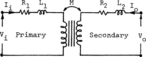
Example 3-5. Identify the z parameters for the transformer shown in Fig. 3-18.

Solution: The induced voltages υ₁ and υ₂ of a transformer due to the currents i₁ in the primary coil and i₂ in the secondary are

$\begin{array}{lll}{\upsilon }_2=M\frac{d{i}_1}{dt}\hfill & \text{and}\hfill & {\upsilon }_1=M\frac{d{i}_2}{dt}\hfill \end{array}$

where M is the mutual inductance between the coils. The loop equations for the primary and the secondary coils are

$\begin{array}{ll}{\upsilon }_1\hfill & =R_1{i}_i+L_1\frac{d{i}_i}{dt}+M\frac{d{i}_o}{dt}\hfill \\ {\upsilon }_o\hfill & =M\frac{d{i}_i}{dt}+R_2{i}_o+L_2\frac{d{i}_o}{dt}\hfill \end{array}$

FIGURE 3-18 Transformer: an example of z parameters.

For ac operation, jω is substituted for the time derivatives (see Sec. A-6, App. A). Thus

$\begin{array}{lll}{V}_i\hfill & =\hfill & \left(R_1+j\omega L_1\right)I_{\iota }+\left(j\omega M\right)I_o\hfill \\ V_o\hfill & =\hfill & \left(j\omega M\right)I_i+\left(R_2+j\omega L_2\right)I_o\hfill \end{array}$

The parameters in the equations above can be compared with the z’s in Eq. 3-27. The z’s are complex numbers. Correspondingly, the V’s and I’s are phasors.

2.  Y Parameters

When the voltages are selected as independent variables, the parameters are admittances or y parameters. From the equations

$\begin{array}{lll}{I}_i=f_1\left(V_i,V_o\right)\hfill & \text{and}\hfill & I_o=f_2\left(V_i,V_o\right)\hfill \end{array}$

we obtain

$\begin{array}{ll}\begin{array}{l}{I}_i=y_i{V}_i+y_r{V}_o\hfill \\ I_o=y_f{V}_i+y_o{V}_o\hfill \end{array}\hfill & \begin{array}{llll}\left[\begin{array}{l}{I}_i\hfill \\ I_o\hfill \end{array}\right]\hfill & =\hfill & \left[\begin{array}{ll}{y}_i\hfill & y_r\hfill \\ y_f\hfill & y_o\hfill \end{array}\right]\hfill & \left[\begin{array}{l}{V}_i\hfill \\ V_o\hfill \end{array}\right]\hfill \end{array}\hfill \end{array}$

(3-29)

where

$\begin{array}{ll}{y}_i={\frac{I_i}{V_i}|}_{V_o=0}\hfill & y_r={\frac{I_i}{V_o}|}_{V_i=0}\hfill \\ y_f={\frac{I_o}{V_{\iota }}|}_{V_o=o}\hfill & y_o={\frac{I_o}{V_o}|}_{V_i=0}\hfill \end{array}$

(3-30)

The y parameters are measured under short-circuit conditions; that is, either V_ι = 0 or V_o = 0. Their interpretation follows that of the z parameters. Admittance is the reciprocal of impedance, and the compliance of a spring is the reciprocal of its stiffness. This does not mean that the y’s in Eq. 3-30 are the reciprocals of the corresponding z’s in Eq. 3-28. The 2 × 2 matrix for the admittances, however, is the inverse of the 2 × 2 matrix for the impedances.

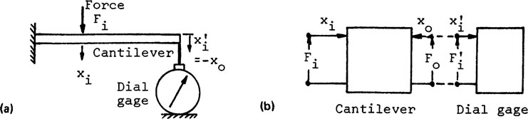
Example 3-6. A cantilever as a force transducer is shown in Fig. 3-19a. The displacement at the end of the cantilever is sensed by means of a dial gage, the model of which is a weak spring (see Fig. 2-20). (a) Derive the equations for the system, assuming zero loading. (b) Repeat by including loading due to the dial gage.

Solution: (a)  The cantilever is modeled as a two-port device as shown in Fig. 3-19b. Since a displacement is the desired output, the appropriate equations are expressed in terms of compliance or influence coefficients [10].

$\begin{array}{l}{x}_{\iota }={\text{δ}}_i{F}_i+{\text{δ}}_r{F}_o\hfill \\ x_o={\text{δ}}_f{F}_i+{\text{δ}}_o{F}_o\hfill \end{array}$

(3-31)

where the x’s are displacements and F’s the forces. The compliances δ’s are defined as

$\begin{array}{ll}{\text{δ}}_i={\frac{x_i}{F_i}|}_{F_o=0}\hfill & {\text{δ}}_r={\frac{x_i}{F_o}|}_{F_i=0}\hfill \\ {\text{δ}}_f={\frac{x_o}{F_i}|}_{F_o=0}\hfill & {\text{δ}}_o={\frac{x_o}{F_o}|}_{F_i=0}\hfill \end{array}$

The equations above are analogous to Eqs. 3-29 and Eqs. 3-30, where the displacement x is analogous to the flow I, and the force F to the potential V. The dial gage is modeled as a one-port. Since the cantilever and the dial gage are in contact, we have $x_i^{\prime }=-x_0\text{ and }{F}_i^{\prime }=F_0,$ as shown in Fig. 3-19b.

FIGURE 3-19 Force measurement: an example of y parameter. (a) System. (b) Model.

For zero loading, the force $F_i^{\prime }$ to deflect the gage becomes zero, and the cantilever is very stiff. The first condition requires δ_rF_o = 0 and δ_oF_o = 0. Hence Eq. 3-31 becomes

$\begin{array}{lll}{x}_{\iota }={\text{δ}}_{\text{ι}}{F}_i\hfill & \text{and}\hfill & x_o={\text{δ}}_f{F}_i\hfill \end{array}$

The second condition requires the compliance δ_ι = 0. Thus the equations reduce further to that for the information model.

$x_o={\text{δ}}_f{F}_i$

(3-32)

(b)  Now consider the loading due to the force for deflecting the dial gage. The equations for the gage are

$\begin{array}{lll}{\text{δ}}_m=\frac{{x^{\prime }}_i}{{F^{\prime }}_{\text{ι}}}=\frac{-x_o}{F_o}\hfill & \text{or}\hfill & F_o=-\frac{x_o}{{\text{δ}}_m}\hfill \end{array}$

where δ_m is the compliance of the spring in the gage. Substituting F_o into the second equation in Eq. 3-31 gives

$\begin{array}{lll}{x}_o={\text{δ}}_f{F}_i-\frac{{\text{δ}}_o}{{\text{δ}}_m}{x}_o\hfill & \text{or}\hfill & x_o=\frac{1}{1+{\text{δ}}_o/{\text{δ}}_m}\left({\text{δ}}_f{F}_i\right)\hfill \end{array}$

(3-33)

Since x_o = δ_fF_ι is the ideal output, the loading is due to the term δ_o/δ_m in Eq. 3-33. Note that Eq. 3-33 is identical to Eq. 3-24 for displacement measurements, where k_m/k_o = δ_o/δ_m, k_m is th stiffness of the spring in the dial gage, and k_o is the stiffness of the cantilever measured at the location of the dial gage.

3.  ABCD Parameters

The analysis of components in cascade can be simplified by means of the ABCD parameters using a recurrence formula in matrix algebra. The technique can be used conveniently for complex arrangements of components in a system [11]. The sign of the current at the output in Fig. 3-20 is reversed for convenience.

When the output variables V_o and I_o are assumed independent, the parameters are the ABCD parameters.

$\begin{array}{ll}\begin{array}{l}{V}_{\mathrm{\iota }}=A{V}_o+B{I}_o\hfill \\ I_i=C{V}_o+D{I}_o\hfill \end{array}\hfill & \begin{array}{llll}\left[\begin{array}{l}{V}_{\text{ι}}\hfill \\ I_i\hfill \end{array}\right]\hfill & =\hfill & \left[\begin{array}{ll}A\hfill & B\hfill \\ C\hfill & D\hfill \end{array}\right]\hfill & \left[\begin{array}{l}{V}_o\hfill \\ I_o\hfill \end{array}\right]\hfill \end{array}\hfill \end{array}$

(3-34)

The recurrence formula above shows that the output of a preceding component is the input to the following component. For two adjacent components, we have $I_i^{\prime }=I_o$ and $V_i^{\prime }=V_o.$.

FIGURE 3-20 Examples of ABCD and mixed parameters. (a) Circuit com ponents in cascade. (b) Transducers in cascade.

$\begin{array}{llll}\left[\begin{array}{l}{V}_i\hfill \\ I_i\hfill \end{array}\right]\hfill & =\left[\begin{array}{ll}A\hfill & B\hfill \\ C\hfill & D\hfill \end{array}\right]\left[\begin{array}{l}{V}_o\hfill \\ I_o\hfill \end{array}\right]\hfill & \left[\begin{array}{l}{V^{\prime }}_{\iota }\hfill \\ {I^{\prime }}_{\iota }\hfill \end{array}\right]\hfill & =\left[\begin{array}{ll}{A}^{\prime }\hfill & B^{\prime }\hfill \\ C^{\prime }\hfill & D^{\prime }\hfill \end{array}\right]\left[\begin{array}{l}{V^{\prime }}_o\hfill \\ {I^{\prime }}_o\hfill \end{array}\right]\hfill \\ \left[\begin{array}{l}{V}_i\hfill \\ I_i\hfill \end{array}\right]\hfill & =\left[\begin{array}{ll}A\hfill & B\hfill \\ C\hfill & D\hfill \end{array}\right]\left[\begin{array}{ll}{A}^{\prime }\hfill & B^{\prime }\hfill \\ C^{\prime }\hfill & D^{\prime }\hfill \end{array}\right]\hfill & \left[\begin{array}{l}{V^{\prime }}_o\hfill \\ {I^{\prime }}_o\hfill \end{array}\right]\hfill & =\left[\begin{array}{ll}A{A}^{\prime }+B{C}^{\prime }\hfill & A{B}^{\prime }+B{D}^{\prime }\hfill \\ C{A}^{\prime }+D{C}^{\prime }\hfill & C{B}^{\prime }+D{D}^{\prime }\hfill \end{array}\right]\left[\begin{array}{l}{V^{\prime }}_o\hfill \\ {I^{\prime }}_o\hfill \end{array}\right]\hfill \end{array}$

(3-35)

The ABCD parameters can readily be related to the other parameters. For example, when the y parameters are redefined according to the sign convention above, we get

$\begin{array}{l}{I}_i=y_i{V}_i-y_r{V}_o\hfill \\ I_o=y_f{V}_i-y_o{V}_o\hfill \end{array}$

(3-36)

It can be shown by simple algebra that

$\begin{array}{ll}A=\frac{y_o}{y_f}\hfill & B=\frac{y_i{y}_o}{y_f}-y_r\hfill \\ C=\frac{1}{y_f}\hfill & D=\frac{y_{\iota }}{y_f}\hfill \end{array}$

(3-37)

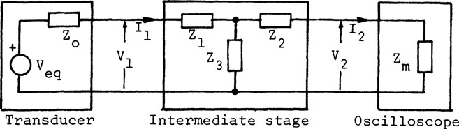
Example 3-7. The schematic of a measuring system is shown in Fig. 3-21. Compare the true output voltage V₁ of the transducer with the measured voltage V₂.

Solution: The open-circuit voltage V_eq is the true output voltage. The loop equation at the transducer output is

FIGURE 3-21 Components in cascade.

$\begin{array}{lll}{V}_{\text{eq}}=I_1{Z}_o+V_1\hfill & \text{or}\hfill & \begin{array}{llll}\left[\begin{array}{l}{V}_{\text{eq}}\\ I_1\end{array}\right]\hfill & =\hfill & \left[\begin{array}{ll}1\hfill & Z_o\hfill \\ 0\hfill & 1\hfill \end{array}\right]\hfill & \left[\begin{array}{l}{V}_1\\ I_1\end{array}\right]\hfill \end{array}\hfill \end{array}$

(3-38)

The loop equations for the intermediate stage are

$\begin{array}{ll}\begin{array}{l}{V}_1=\left(Z_1+Z_3\right)I_1-Z_3{I}_2\\ V_2=Z_3{I}_1-\left(Z_2+Z_3\right)I_2\end{array}\hfill & \begin{array}{llll}\left[\begin{array}{l}{V}_1\\ I_1\end{array}\right]\hfill & =\hfill & \left[\begin{array}{ll}A\hfill & B\hfill \\ C\hfill & D\hfill \end{array}\right]\hfill & \left[\begin{array}{l}{V}_2\\ I_2\end{array}\right]\hfill \end{array}\hfill \end{array}$

(3-39)

where

$\begin{array}{ll}A=\frac{Z_1+Z_2}{Z_3}\hfill & B=\frac{Z_1{Z}_2+Z_2{Z}_3+Z_3{Z}_1}{Z_3}\hfill \\ C=\frac{1}{Z_3}\hfill & D=\frac{Z_2+Z_3}{Z_3}\hfill \end{array}$

The loop equation at the input of the oscilloscope is

$\begin{array}{lll}{V}_2=I_2{Z}_m\hfill & \text{or}\hfill & I_2=\frac{V_2}{Z_m}\hfill \end{array}$

(3-40)

Substituting Eqs. 3-39 and 3-40 into Eq. 3-38, we get

$\left[\begin{array}{l}{V}_{\text{eq}}\\ I_1\end{array}\right]=\left[\begin{array}{ll}1\hfill & Z_o\hfill \\ 0\hfill & 1\hfill \end{array}\right]\hspace{0.17em}\left[\begin{array}{ll}A\hfill & B\hfill \\ C\hfill & D\hfill \end{array}\right]\hspace{0.17em}\left[\begin{array}{l}{V}_2\\ V_2/Z_m\end{array}\right]$

Multiplying out the matrices and simplifying, we obtain

$\frac{V_2}{V_{\text{eq}}}=\frac{Z_3{Z}_m}{Z_o\left(Z_2+Z_3\right)+\left(Z_1{Z}_2+Z_2{Z}_3+Z_3{Z}_1\right)+Z_m\left(Z_0+Z_1+Z_2\right)}$

4.  Mixed Parameters

Three of the six possible descriptions of two-port devices are presented above. The remaining three are the A′B′C′D′, g, and hybrid parameters. These will not be discussed here, since the A′B′C′D′ and g parameters are similar to the ABCD and hybrid parameters. Hybrid parameters are examined in detail in the next section. The general case of mixed parameters is illustrated in the example to follow.

Example 3-8. Two transducers in cascade are shown in Fig. 3-20b. The functional relations of the components are

$\begin{array}{lll}\left[\begin{array}{l}{y}_1\\ x_2\end{array}\right]=\left[\begin{array}{ll}M\hfill & N\hfill \\ P\hfill & Q\hfill \end{array}\right]\left[\begin{array}{l}{x}_1\\ y_2\end{array}\right]\hfill & \text{and}\hfill & \left[\begin{array}{l}{y^{\prime }}_1\\ {x^{\prime }}_2\end{array}\right]=\left[\begin{array}{ll}{M}^{\prime }\hfill & N^{\prime }\hfill \\ P^{\prime }\hfill & Q^{\prime }\hfill \end{array}\right]\left[\begin{array}{l}{x^{\prime }}_1\\ {y^{\prime }}_2\end{array}\right]\hfill \end{array}$

Find the overall relation between $\left(y_1^{\prime },x_2\right)\text{ and }\left(x_1,y_2^{\prime }\right).$

Solution: Since $x_1^{\prime }=y_1\text{ and }{x}_2^{\prime }=y_2,$ we get

$\begin{array}{lll}\begin{array}{l}{y}_1-N{y}_2=M{x}_1\\ x_2-Q{y}_2=P{x}_1\end{array}\hfill & \text{and}\hfill & \begin{array}{l}{y^{\prime }}_1-M^{\prime }{y}_1=N^{\prime }{y^{\prime }}_2\\ y_2-P^{\prime }{y}_1=Q^{\prime }{y^{\prime }}_2\end{array}\hfill \end{array}$

Expressing the equations in matrices, we have

$\begin{array}{l}\left[\begin{array}{llll}1\hfill & -N\hfill & 0\hfill & 0\hfill \\ 0\hfill & -Q\hfill & 1\hfill & 0\hfill \\ -M^{\prime }\hfill & 0\hfill & 0\hfill & 1\hfill \\ -P^{\prime }\hfill & 1\hfill & 0\hfill & 0\hfill \end{array}\right]\hspace{0.17em}\left[\begin{array}{l}{y}_1\\ y_2\\ x_2\\ {y^{\prime }}_1\end{array}\right]=\left[\begin{array}{llll}M\hfill & 0\hfill & 0\hfill & 0\hfill \\ P\hfill & 0\hfill & 0\hfill & 0\hfill \\ 0\hfill & 0\hfill & N^{\prime }\hfill & 0\hfill \\ 0\hfill & 0\hfill & Q^{\prime }\hfill & 0\hfill \end{array}\right]\hspace{0.17em}\left[\begin{array}{l}{x}_1\\ 0\\ {y^{\prime }}_2\\ 0\end{array}\right]\hfill \\ \left[\begin{array}{l}{y}_1\\ y_2\\ x_2\\ {y^{\prime }}_1\end{array}\right]={\left[\begin{array}{lll}1\hfill & -N\hfill & 0\hfill \\ 0\hfill & -Q\hfill & 1\hfill \\ -M^{\prime }\hfill & 0\hfill & 0\hfill \\ -P^{\prime }\hfill & 1\hfill & 0\hfill \end{array}\right]}^{-1}\left[\begin{array}{llll}M\hfill & 0\hfill & 0\hfill & 0\hfill \\ P\hfill & 0\hfill & 0\hfill & 0\hfill \\ 0\hfill & 0\hfill & N^{\prime }\hfill & 0\hfill \\ 0\hfill & 0\hfill & Q^{\prime }\hfill & 0\hfill \end{array}\right]\left[\begin{array}{l}{x}_1\\ 0\\ {y^{\prime }}_2\\ 0\end{array}\right]\hfill \end{array}$

It can be shown by simple algebra that the desired overall relation is

$\begin{array}{lll}\left[\begin{array}{l}{y^{\prime }}_1\\ x_2\end{array}\right]\hfill & =\hfill & \frac{1}{1-N{P}^{\prime }}\hfill \\ \hfill & \hfill & \times \left[\begin{array}{ll}M{M}^{\prime }\hfill & \left[N^{\prime }\left(1-N{P}^{\prime }\right)+M^{\prime }N{Q}^{\prime }\right]\hfill \\ \left[M{P}^{\prime }Q+P\left(1-N{P}^{\prime }\right)\right]\hfill & Q{Q}^{\prime }\hfill \end{array}\right]\left[\begin{array}{l}{x}_1\\ {y^{\prime }}_2\end{array}\right]\hfill \end{array}$

D.  Three-Port Devices: Amplifiers

A three-port device has three ports for energy transfer, as shown in Figs. 2-15b and 2-18b. It represents a non-self-generating transducer as well as an intermediate component in a measuring system, such as a modulator or an amplifier. Signal modulation is described in Chapter 5. The transistor amplifier is examined in this section, which also provides background for some of the laboratory exercises.

An amplifier is a three-port device. The signal input controls the power supply or an energy source to deliver an output at the desired amplitude or power level. It is expedient to simplify the amplifier as a two-port with controlled sources 12]. The incremental model of a three-port shown in Fig. 2-18b has six variables. Only three of the six variables can be independent. This gives a set of three simultaneous equations, as shown in Eq. 2-33. It can be shown that there exist 20 sets of such simultaneous equations for describing the same system, resulting in a total of 20 × 9 = 180 parameters. The problem becomes unwieldy.

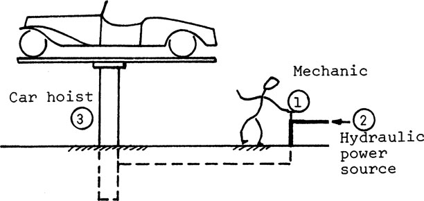
The hydraulic amplifier in the form of a car hoist shown in Fig. 3-22 is an example of a controlled-source device. The mechanic regulates the valve at location 1 to control the hydraulic power at location 2 for hoisting the car at location 3. The hoist is a three-port. Since the hydraulic supply is constant, the model of the hoist is a two-port with a controlled source. When the input signal is applied, the output follows the input but at a much higher power level.

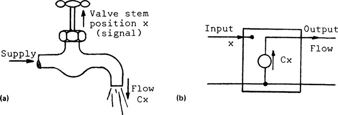
A controlled source device can be unilateral or bilateral. The household spigot shown in Fig. 3-23 is modeled as unilateral with a controlled flow source. The input is the valve stem position x, the controlled source is a flow generator, and the output is the flow. The flow delivered Cx is controlled by x, where C is a constant. The device is unilateral, because the flow does not influence the valve stem position. Thus the input x is left “dangling” in the model. An engine dynanometer with a dc generator for power absorption is bilateral. The generator can also operate as a dc motor for starting the engine or for finding its frictional horsepower. This is a special of bilateral devices. Normally, the forward and reverse characteristics are not alike.

A simple transistor amplifier will be described as a typical controlled source device. The topics will include static characteristics (see Sec. 2-2A), determining the operating point, and linearization about the operation point for obtaining the dynamic model (see Secs. 2-2E and 2-3C). Except for the terminology, most of the principles were presented in previous sections.

FIGURE 3-22 Hydraulic power amplifier.

FIGURE 3-23 Example of unilateral controlled source. (a) Spigot. (b) Idealized model with controlled source, Cx.

1.  Static Characteristics of Transistors [13]

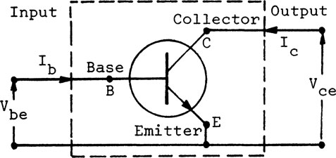
A transistor has three terminals. It is either the NPN or the PNP type. The symbol of a NPN transistor is shown in Fig. 3-24. The terminals are labeled as the base B, collector C, and emitter E. The arrow on the emitter points toward the direction of the flow of positive charges from P to N. The arrow would point in the opposite direction for a PNP transistor. Any one of the three terminals can be used as common lead in a circuit. The common-emitter configuration in the figure is often used for a general-purpose amplifier.

The static characteristics give the functional relations for the variables. The input variables in Fig. 3-24 are the base current I_b, and the input voltage V_be, where the first subscript (b) denotes the base and the second subscript (e) the common-emitter configuration. The output variables are the collector current I_c and the output voltage V_ce, where c denotes the collector. Choosing I_b and V_ce as independent, we get

FIGURE 3-24 NPN transistor with common emitter.

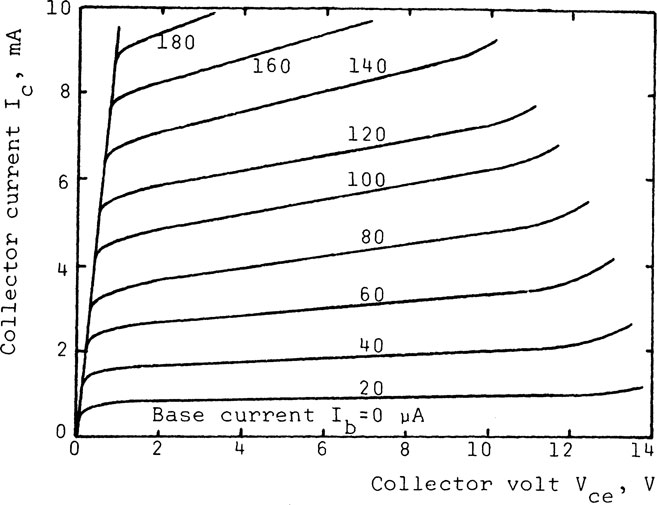
FIGURE 3-25 Typical static characteristics of NPN transistor.

$\begin{array}{l}{I}_c=f_1\left(V_{ce},I_b\right)\hfill \\ V_{be}=f_2\left(V_{ce},I_b\right)\hfill \end{array}$

(3-41)

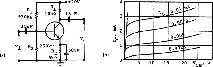
The characteristics curves described by the first equation above are illustrated in Fig. 3-25. The second equation can be approximated and the curves are not shown.

2.  Operating Point

The operating point Q of an ac amplifier is a quiescient point defined by its initial conditions. The ac signals are dynamic quantities, while the initial conditions are dc quantities determined from dc circuit analysis. Hence all ac quantities can be neglected in order to establish Q.

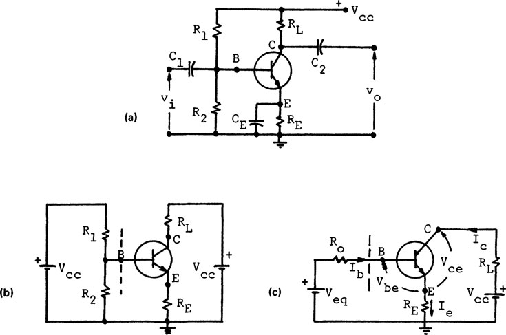
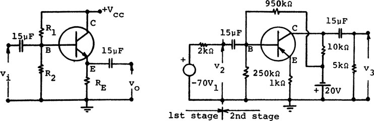
The circuit of a common-emitter ac amplifier is shown in Fig. 3-26a. The procedure for finding Q is to reduce the circuit to a corresponding dc circuit shown in Fig. 3-26b. First, the ac input and output voltages υ_i and υ_o are neglected. Second, the capacitors are omitted, since they do not influence the dc analysis. Finally, the battery V_cc is shown explicitly by connecting its negative terminal to ground. The dc circuit is further simplified in Fig. 3-26c by reducing the part to the left of B (dashed line) by its Thevenin’s equivalent, where

FIGURE 3-26 Method to find operating point. (a) Common-emitter amplifier. (b) Omitting ac components. (c) To find operating point.

$\begin{array}{lll}{R}_o=\frac{R_1{R}_2}{R_1+R_2}\hfill & \text{and}\hfill & V_{\text{eq}}=\frac{R_2}{R_1+R_2}{V}_{cc}\hfill \end{array}$

(3-42)

The transistor is a junction, and the node equation for the currents at the transistor in Fig. 3-26c is

$\begin{array}{lll}{I}_b+I_c-I_e=0\hfill & \text{or}\hfill & I_c\simeq I_e\hfill \end{array}$

(3-43)

Since I_b is the input signal for controlling I_c, I_b ≪ I_c. The approximation is also evident from the characteristics shown in Fig. 3-25, where I_c is of the order of milliamperes and I_b is of microamperes.

Since I_c = I_e, the equation for the collector loop on the right side of Fig. 3-26c is

$V_{cc}=\left(R_L+R_E\right)I_c+V_{ce}$

(3-44)

or

$I_c=\underset{\text{slope}}{\underbrace{\left(-\frac{1}{R_L+R_E}\right)}}{V}_{ce}+\underset{\text{constant}}{\underbrace{\frac{1}{R_L+R_E}}}{V}_{cc}$

(3-45)

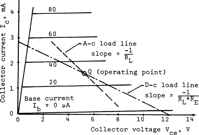
This gives the dc load line [14] shown in Fig. 3-27. Voltages and currents in the collector loop must vary along this line, because they are governed by the loop equation.

The equation for the base loop of Fig. 3-26c is

$V_{\text{eq}}=R_0{I}_b+V_{be}+R_E{I}_c$

(3-46)

where V_be is about 0.2 V for germanium and 0.6 V for silicon transistor. Eliminating I_c between Eqs. 3-44 and 3-46 gives

$V_{ce}=\underset{\text{slope}}{\underbrace{\left[R_0\left(1+\frac{R_L}{R_E}\right)\right]}}{I}_b+\underset{\text{constant}}{\underbrace{\left[V_{cc}-\left(V_{\text{eq}}-V_{be}\right)\left(1+\frac{R_L}{R_E}\right)\right]}}$

(3-47)

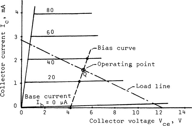
FIGURE 3-27 Locating the operating point Q.

This gives the equation of the bias curve shown in Fig. 3-27. The intersection of the dc load line and the bias curve gives the operating point Q.

In summary, the plot in Fig. 3-27 has three variables, I_c, V_ce, and I_b. The collector loop gives the load line, which relates I_c and V_ce. The base loop gives the bias curve, which relates V_ce and I_b. The intersection of the two lines gives the operating point Q.

3.  Dynamic Modeling

The dynamic model is obtained from the static characteristics shown in Fig. 3-27 by means of linearization about Q (see Sec. 2-2E). In this section we describe the process of voltage amplification for background information, obtain a controlled-source model for the transistor, reduce the amplifier circuit to its ac equivalent, and deduce the equations for an ac amplifier.

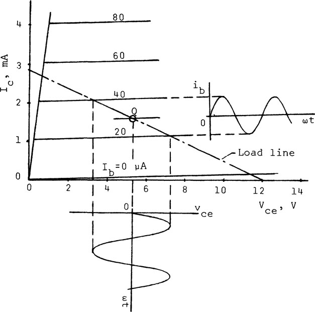
The process of ac voltage amplification is illustrated for the amplifier shown in Fig. 3-26a. Let the ac output voltage υ_o be controlled by the ac base current i_b. Assume that i_b is sinusoidal and fluctuating between 20 and 40 μA about Q, as shown in Fig. 3-28. Thus the projections of i_b on the load line gives the corresponding values of i_c and v_ce about Q. The ac output voltage is υ_o = v_ce. For the given illustration, the peak-to-peak value of i_b is 20 μA, and the corresponding v_o is approximately (7.2 – 5.2) = 4 V_p-p. It will be shown that the dc load line should be replaced by an ac load line for the ac amplifier.

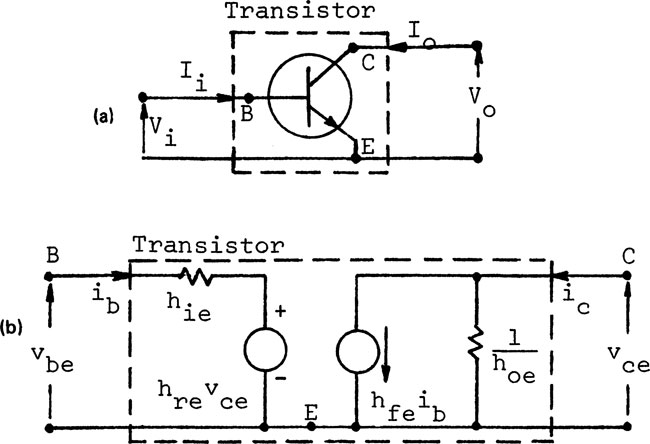
The controlled-source model of a common-emitter amplifier is shown in Fig. 3-29. The subscripts i and o denote the input and output quantities. Conforming to standard notations, we define V_i = V_be, I_i = I_b, V_o = V_ce, and I_o = I_c. Let the V’s and I’s be related by

$\begin{array}{l}{V}_{be}=f_1\left(I_b,V_{ce}\right)\hfill \\ I_c=f_2\left(I_b,V_{ce}\right)\hfill \end{array}$

The incremental model and the controlled sources are deduced from the equations above.

$\begin{array}{lll}{\upsilon }_{be}\hfill & =\hfill & h_{ie}{i}_b+h_{re}{\upsilon }_{ce}\hfill \\ i_c\hfill & =\hfill & h_{fe}{i}_b+h_{oe}{\upsilon }_{ce}\hfill \end{array}$

(3-48)

where

$\begin{array}{ll}{h}_{ie}={\frac{V_{be}}{I_b}|}_{V_{ce}=0}\hfill & h_{re}={\frac{V_{be}}{V_{ce}}|}_{I_b=0}\hfill \\ h_{fe}={\frac{I_c}{I_b}|}_{V_{ce}=0}\hfill & h_{oe}={\frac{I_c}{V_{ce}}|}_{I_b=0}\hfill \end{array}$

(3-49)

FIGURE 3-28 Amplifying process.

The h’s are the hybrid parameters. The subscript i is for input, r for reverse, f for forward, and o for output. The subscript e denotes the common emitter. The parameters are mixed dimensionally; h_ie has the dimension of impedance, h_oe admittance, h_fe a current ratio, and h_re a voltage ratio. Note that the model has two controlled sources, shown in Fig. 3-29b. The input current i_b controls the current generator h_fei_b at the output, and the output voltage v_ce controls the voltage generator h_re v_ce at the input.

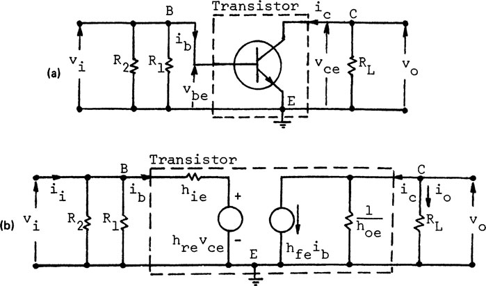
The ac equivalent circuit is deduced from the circuit in Fig. 3-26a by omitting all components that do not affect the ac operation. First, all capacitors are replaced with short circuits. The purpose of the capacitors C₁, C₂, and C_E is to block the dc in the circuit. They offer low-impedance paths for the high-frequency ac signals. Second, V_cc offers a low-impedance path for the ac signals, and the terminal +V_cc is connected directly to ground in the ac circuit. Thus the components remaining in the ac equivalent circuit are the transistor, R₁, R₂, and R_L, as shown in Fig. 3-30a. Finally, substituting the hybrid model from Fig. 3-29b for the transistor, we obtain the ac equivalent circuit in Fig. 3-30b.

FIGURE 3-29 Hybrid model of transistor. (a) Common-emitter. (b) Hybrid parameters.

Equations for the ac amplifier are deduced from the circuit shown in Fig. 3-30b. The loop equation at the input is

${\upsilon }_i=h_{ie}{i}_b+h_{re}{\upsilon }_{ce}$

(3-50)

Since υ_i is applied across B and E, R₁ and R₂ do not affect the equation. The node equation at the output C is

$i_o+i_c=0$

Substituting i_c = h_fei_b + h_oeυ_ce and i_o = υ_o/R_L, we obtain

$\frac{{\upsilon }_o}{R_L}+h_{oe}{\upsilon }_o+h_{fe}{i}_b=0$

(3-51)

The open-circuit voltage gain is υ_o/υ_i. Eliminating i_b between Eqs. 3-50 and 3-51 yields

FIGURE 3-30 Ac equivalent circuit of transistor amplifier. (a) Ac circuit—common emitter amplifier. (b) Ac equivalent circuit—common emitter amplifier.

$\frac{{\upsilon }_o}{{\upsilon }_{\iota }}=\frac{-1}{h_{ie}\left(1+h_{oe}{R}_L\right)/\left(h_{fe}{R}_L\right)-h_{re}}$

(3-52)

The current gain is i_o/i_b. Substituting υ_o = R_Li_o into Eq. 3-51 gives

$\frac{i_o}{i_b}=\frac{-h_{fe}}{1+h_{oe}{R}_L}$

(3-53)

Finally, the dc load line is replaced by an ac load line for ac operation. The collector loop equation from Fig. 3-30a is

$\begin{array}{lll}{\upsilon }_{ce}+i_c{R}_L=0\hfill & \text{or}\hfill & i_c=-\frac{1}{R_L}{\upsilon }_{ce}\hfill \end{array}$

(3-54)

The ac load line goes through the operating point Q with the slope of −1/R_L, as shown in Fig. 3-31. The process of amplification shown in Fig. 3-28 should be modified by using the ac load line instead of the dc load line.

3-4.  BRIDGE CIRCUITS

A bridge denotes a particular arrangement of components in an instrument. It does not pertain to a specific type of hardware. Bridges are used extensively in instrumentation. Bridge circuits for the null balance and unbalance methods of measurement are described in this section.

FIGURE 3-31 To find ac load line.

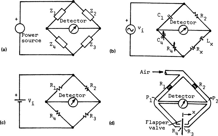
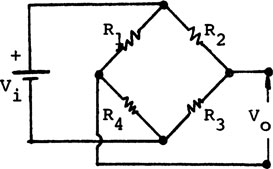
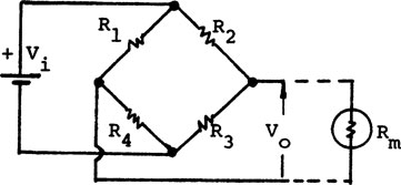
Examples of bridges are shown in Fig. 3-32. The general configuration in Fig. 3-32a consists of four arms of impedances Z₁ to Z₄, a power supply, and a detector. The Owen bridge [15] shown in Fig. 3-32b is for electrical measurements. It does not appear symmetrical compared with the familiar Wheatstone bridge.

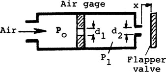
A Wheatstone bridge with strain gages is shown in Fig. 3-32c. The air bridge for measuring the displacement x of the flapper valve, shown in Fig. 3-32d, has orifices R₁ to R₄ instead of strain gages. The air exhausts to the atmosphere to complete the flow circuit. The detector is a sensitive differential pressure transducer or a flow meter (e.g., Hasting-Raydist, Inc., Hampton, Virginia). The bridge is initially balanced for zero differential pressure, or P₁ – P₂ = 0. The displacement x unbalances the bridge by changing R₃ and R₄. thus (P₁ – P₂) ≠ 0, and the value of x is indicated by the detector.

A.  Null Balance Systems

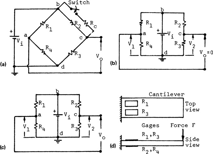
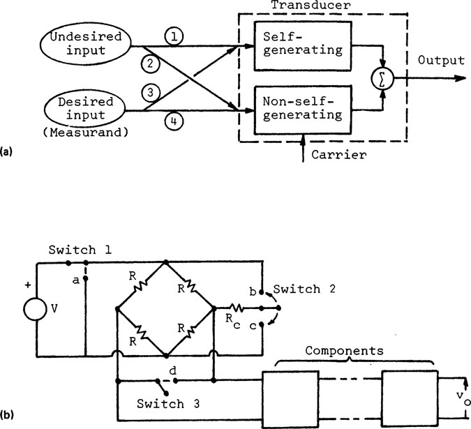
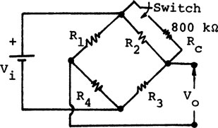
A bridge using the null balance method compares an unknown X₁ with a reference standard X₂ (see Fig. 3-2). The bridge is balanced before and after a measurement. The bridge circuit in Fig. 3-33a is rearranged in Fig. 3-33b as a differential for comparing the voltages V_l and V₂ of two potentiometers. The calibrating resistor R_c will be described later.

FIGURE 3-32 Examples of bridges. (a) Bridge circuit. (b) Owen bridge. (c) Wheatstone bridge. (d) Air bridge.

The R’s in each potentiometer form a voltage divider. The voltages from the circuit are

$\begin{array}{lll}\frac{V_1}{V_i}=\frac{R_4}{R_1+R_4}\hfill & \text{and}\hfill & \frac{V_2}{V_i}=\frac{R_3}{R_2+R_3}\hfill \end{array}$

(3-55)

$V_o=V_2-V_1=\left(\frac{R_3}{R_2+R_3}-\frac{R_4}{R_1+R_4}\right)V_i$

(3-56)

The bridge is balanced when V_o = (V₂ – V₁) = 0. Thus

$\begin{array}{lll}\frac{R_3}{R_2+R_3}=\frac{R_4}{R_1+R_4}\hfill & \text{or}\hfill & R_1{R}_3=R_2{R}_4\hfill \end{array}$

(3-57)

If the components in the bridge are impedances, the corresponding equation is

$Z_1{Z}_3=Z_2{Z}_4$

(3-58)

FIGURE 3-33 Strain gage bridge circuits. (a) Strain gage bridge. (b) Null-balance system. (c) Unbalance system. (d) Force transducer.

The equation does not imply that R₁ = R₂ or R₃ = R₄. It stipulates only the ratio of the R’s. For example, let R₂ be the sensor for the bridge in Fig. 3-33b, and the bridge is initially balanced. An input changes R₁ to R₁ + ΔR₁. At the same time, the reference R₂ is adjusted to become R₂ + ΔR₂ to rebalance the bridge. From Eq. 3-57 we get

$\begin{array}{lll}\left(R_1+\Delta R_1\right)R_3=\left(R_2+\Delta R_2\right)R_4\hfill & \text{or}\hfill & \frac{\Delta R_1}{R_1}=\frac{\Delta R_2}{R_2}\hfill \end{array}$

(3-59)

Since ΔR₂ is known, ΔR₁ and the value of the input can be evaluated.

B.  Unbalance and Differential Systems

For the unbalance method in Fig. 3-33c, one of the potentiometers is for the initial zero adjustment (see Fig. 3-4). Assume that R₁ and R₄ are for this adjustment, and R₂ and R₃ are strain gages in a half bridge with R₂ = R₃. when the bridge is unbalanced by an applied strain, R₂ becomes R₂ + ΔR₂ and R₃ becomes R₃ – ΔR₃. The output voltage V_o is obtained from Eq. 3-56 with the new values of R₂ and R₃.

Alternatively, the R’s in Fig. 3-33c can be used in a full bridge for a differential measurement. Consider a force transducer in the form of a cantilever, shown in Fig. 3-33d, with gages R₁ and R₃ on the top of the cantilever and R₂ and R₄ at the bottom. When the force F is applied, the gages on the top will be under tension and those at the bottom under compression. R₁ and R₃ become R₁ + ΔR₁ and R₃ + ΔR₃, and R₂ and R₄ become R₂ – ΔR₂ and R₄ – ΔR₄, respectively. The corresponding bridge output from Eq. 3-56 is

$V_o=V_2-V_1=\left(\frac{R_3+\Delta R_3}{R_2-\Delta R_2+R_3+\Delta R_3}-\frac{R_4-\Delta R_4}{R_1+\Delta R_1+R_4-\Delta R_4}\right)V_i$

(3-60)

Note that the gages in a bridge are connected such that opposite strains are applied to the adjacent gages. The bridge output is zero if equal strains are applied to adjacent gages. In other words, opposite gages in a bridge must have strains in the same direction.

Example 3-9. The force transducer in Fig. 3-33d consists of a cantilever and a strain gage bridge. Assume that V_ι = 4 V, the gage factor G_f = 2.0, R₁ = R₂ = R₃ = R₄ = R = 120 Ω. If the stress at each gage is 140 MPa (≃ 20,000 psi), find (a) the change in gage resistance, and (b) the output voltage V_o.

Solution: (a)  From G_f = (ΔR/R)/(strain) and stress = (Young’s modulus E)(strain), where E = 200 GPa for steel, we get

$\begin{array}{l}\frac{\Delta R}{R}=G_f\times \text{strain}=G_f\frac{\text{stress}}{E}=2\times \frac{140\text{MPa}}{200\text{GPa}}=1.4\times {10}^{-3}\hfill \\ \Delta R=120\left(1.4\times {10}^{-3}\right)=0.17\Omega \hfill \end{array}$

Note that these ΔR for each gage is only 0.14%.

(b)  Substituting the values in Eq. 3-60, the bridge output V_o due to four active gages is

$\begin{array}{lll}{V}_o\hfill & =\hfill & \left(\frac{120+0.17}{2\times 120}-\frac{120-0.17}{2\times 120}\right)\times 4=\left(1.4\times {10}^{-3}\right)\times 4\hfill \\ \hfill & =\hfill & \begin{array}{lll}5.6\times {10}^{-3}\text{V}\hfill & \text{or}\hfill & 5.6\text{mV}\hfill \end{array}\hfill \end{array}$

Strain gages can be calibrated directly or indirectly. The force transducer in Fig. 3-33d can be calibrated directly by applying a known weight and observing the output V_o. A direct calibration is generally not possible because once a gage is bonded to a surface, it cannot be transferred to another location for calibration. The indirect calibration of a strain gage bridge is shown in Fig. 3-33a. When the gage R₂ and the calibrating resistor R_c are in parallel, the resistance change between the terminals b and c is an equivalent strain applied to R₂.

Example 3-10. Use the data in Example 3-9 for the bridge in Fig. 3-33a. (a) Find R_c to give an equivalent strain of 100 μs (microstrain) and the bridge output V_o during calibration, (b) If the bridge has four active gages and V_o = 2.5 mV, find the strain indicated by the bridge.

Solution: (a)  The resistance for R₂ and R_c in parallel is

$\begin{array}{lll}\frac{R_{c}R}{R_c+R}=\left(R-\Delta R\right)\hfill & \text{or}\hfill & \Delta R=\frac{R^2}{R_c+R}\hfill \end{array}$

From ΔR/R = G_f (strain), we get

$\Delta R=R{G}_f\left(\text{strain}\right)=R\left(2.0\right)\left(100\times {10}^{-6}\right)$

Eliminating ΔR from the equations above gives

$\begin{array}{lll}\frac{R^2}{R_c+R}=R\left(2.0\right)\left(0.0001\right)\hfill & \text{or}\hfill & R_c\simeq 600\text{k}\Omega \hfill \end{array}$

The output voltage V_o is calculated from Eq. 3-60. Since only R₂ is “active” for the calibration, we have

$\begin{array}{lll}\frac{\Delta R}{R}\hfill & =\hfill & \frac{R}{R_c+R}\simeq \frac{R}{R_c}=\frac{120\Omega }{600\text{k}\Omega }=0.20\times {10}^{-3}\hfill \\ \frac{V_o}{V_i}\hfill & =\hfill & \frac{R}{R-\Delta R+R}-\frac{R}{R+R}=\frac{1}{2}\left(\frac{1}{1-\Delta R/2R}-1\right)\hfill \\ \hfill & =\hfill & \frac{1}{2}\left[1+\frac{\Delta R}{2R}+{\left(\frac{\Delta R}{2R}\right)}^2+\cdots -1\right]\hfill \\ \hfill & \simeq \hfill & \begin{array}{lll}\frac{1}{2}\frac{\Delta R}{2R}\hfill & \text{or}\hfill & V_o=\frac{1}{2}\left(\frac{0.2\times {10}^{-3}}{2}\right)\times 4=0.2\text{mV}\hfill \end{array}\hfill \end{array}$

(b)  The bridge uses one “active” gage for its calibration. If the bridge uses four active gages, V_o is four times that of a single gage. In other words, the actual strain is one-fourth of that indicated by V_o of 2.5 mV. Since 100 microstrain during calibration gives 0.2 mV, we have

$\text{Strain}=\frac{1}{4}\left(\frac{2.5\text{mV}}{0.2\text{mV}}\right)100\text{μstrian}=313\text{μstrain}$

A bridge constant C_b is used for finding the actual strain in a bridge when only one gage is used for the calibration.

$C_b=\frac{\text{actual bridge output}}{\text{output if only one active gage}}$

(3-61)

The bridge constant for Example 3-10 is C_b = 4, because the bridge has four active gages and only one gage is used for its calibration.

A high-impedance voltmeter is generally used for measuring V_o at the bridge output, and loading is minimal. Loading should be considered when a low-impedance detector, such as a galvanometer, is used for measuring V_o.

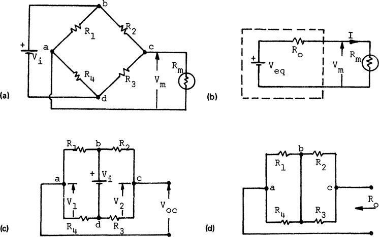
Example 3-11. The output of the strain gage bridge shown in Fig. 3-34a is measured with a galvanometer of input impedance R_m = 200 Ω. Using the data from Example 3-9, find (a) the measured voltage V_o at the bridge output, and (b) the deflection of the galvanometer if its sensitivity is 10 μA/cm.

Solution: (a)  The bridge circuit is reduced to its Thévenin’s equivalent in Fig. 3-34b. The open-circuit voltage in Fig. 3-34c is V_oc = V_eq = 5.6 mV from Example 3-9. The output impedance R_o is the impedance of the bridge with all energy sources removed. The voltage V_i in Fig. 3-34c is removed by replacing with a short circuit, as shown in ig. 3-34d. Thus R_o is the series combination of R₁ and R₄ in parallel and R₂ and R₃ in parallel.

FIGURE 3-34 Thévenin’s equivalent of bridge circuit. (a) Strain gage bridge. (b) Thévenin’s equivalent. (c) To find V_eq. (d) To find R_o.

$\begin{array}{lll}{R}_o\hfill & =\hfill & \frac{R_1{R}_4}{R_1+R_4}+\frac{R_2{R}_3}{R_2+R_3}=\frac{\left(R+\Delta R\right)\left(R-\Delta R\right)}{R+\Delta R+R-\Delta R}\hfill \\ \hfill & \hfill & +\frac{\left(R-\Delta R\right)\left(R+\Delta R\right)}{R-\Delta R+R+\Delta R}\hfill \\ \hfill & \simeq \hfill & R=120\Omega \hfill \end{array}$

Since ΔR/R is small, R_o is approximately 120 Ω. From the Thévenin’s equivalent in Fig. 3-34b, R_m and R_o form a voltage divider for V_eq. The measured voltage is

$V_m=\frac{R_m}{R_m+R_o}-V_{\text{eq}}=\frac{200}{200+120}\times 5.6\text{mV}=3.5\text{mV}$

(b)  The current I through the galvanometer in Fig. 3-34b is

$I=\frac{V_m}{R_m}=\frac{3.5\text{mV}}{200\Omega }=1.75\text{μA}$

Hence the deflection of the galvanometer is 1.75 cm.

3-5.  BASIC TRANSDUCER CIRCUITS

Transducers are self-or non-self-generating. Methods for driving non-self-generating transducers are examined in this section. Self-generating transducers do not require external power sources and are not a part of this discussion.

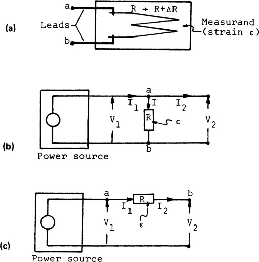
A resistance strain gage is used to represent typical non-self-generating transducer for this discussion. The gage of resistance R shown in Fig. 3-35a can be placed either in parallel or in series with an ideal power source, as shown in Fig. 3-35b and c. It is assumed that (1) an output voltage due to the applied strain is measured with a voltmeter of high input impedance, that is, the voltmeter is essentially an open circuit, and (2) an output current is measured with an ammeter of low input impedance, that is, the ammeter is essentially a short circuit.

A.  Ideal Power Sources

An ideal power source is either a voltage or a current source (see Table A-1 in Appendix A). The strain gage can be placed either in parallel or in series with an ideal power source, as shown in Fig. 3-35b and Fig. 3-35c, respectively. For both cases the quantities available for measurement are the voltages V₁ and V₂ and the currents I₁ and I₂.

For the parallel circuit with an ideal voltage source V_i shown in Fig. 3-35b, an ammeter to measure I₂ will short circuit the gage. Hence I₂ cannot be used. Since V₁ = V₂ = V_i = constant, the voltages cannot be used. Thus only I₁ can be used for measuring the applied strain in the gage. The equations from the corresponding circuit in Fig. 3-36a are

FIGURE 3-35 Non-self-generating transducers with ideal power sources. (a) Non-self-generating transducer. (b) Parallel circuit. (c) Series circuit.

$\begin{array}{lll}{V}_i\hfill & =\hfill & \begin{array}{lll}RI\hfill & \text{and}\hfill & V_i=\left(R+\Delta R\right)\left(I+\Delta I\right)\hfill \end{array}\hfill \\ V_i\hfill & =\hfill & RI+I\Delta R+\Delta I\left(R+\Delta R\right)\hfill \\ \Delta I\hfill & =\hfill & \frac{-I\Delta R}{R+\Delta R}=-\frac{V_{\iota }}{R}\frac{\Delta R/R}{\Delta R/R}\hfill \\ \hfill & =\hfill & -\frac{V_i}{R}\frac{\Delta R}{R}\left[1-\frac{\Delta R}{R}+{\left(\frac{\Delta R}{R}\right)}^2-···\right]\hfill \\ \hfill & \simeq \hfill & -\frac{V_i}{R}\frac{\Delta R}{R}=-\frac{V_i}{R}\left(\text{gage factor}\right)\left(\text{strain}\right)\hfill \end{array}$

(3-62)

Note that the output ΔI in Eq. 3-62 for a constant-voltage drive is inherently nonlinear. The degree of nonlinearity depends on the magnitude of ΔR/R. This is small for metallic strain gages, but can be large for semiconductor gages.

FIGURE 3-36 Possible methods of measurement. Non-self-generating transducer with ideal power sources. (a) Constant-voltage drive. (b) Constant-current drive.

For the parallel circuit in Fig. 3-35b with an ideal current source I_i, I₂ will short circuit the gage. Since I₁ = I_i = constant, only V₁ = V₂ can be used for measuring the strain in the gage. The equations from the corresponding circuit in Fig. 3-36b are

$\begin{array}{lll}V=R{I}_i\hfill & \text{and}\hfill & V+\Delta V=\left(R+\Delta R\right)I_i=R{I}_{\iota }+\Delta R{I}_{\iota }\hfill \\ \Delta V=I_i\Delta R\hfill & \hfill & \hfill \end{array}$

(3-63)

Since the output ΔV is proportional to ΔR in Eq. 3-63, the constant-current drive is inherently linear. This is an advantage when ΔR/R is large.

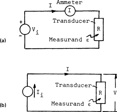
Similarly, ideal power sources can be used for the series circuit shown in Fig. 3-35c. With an ideal voltage source, the only appropriate circuit is that shown in Fig. 3-36a. With an ideal current source, the only appropriate circuit is that shown in Fig. 3-36b.

In summary, the two circuits in Fig. 3-36 are the only possible configurations when a non-self-generating transducer is driven by an ideal voltage or current source [16].

B.  Nonideal Power Sources

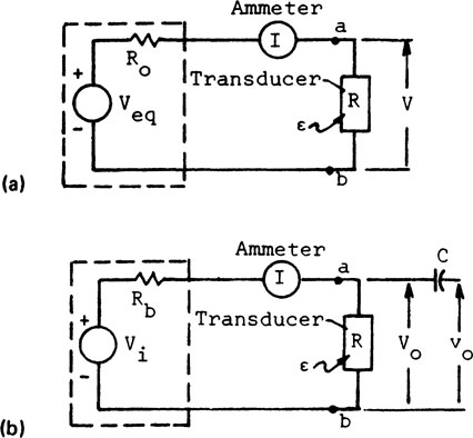
A nonideal power source can be reduced to its Thévenin’s equivalent, shown in Fig. 3-37a, where V_eq, is an ideal voltage source and R_o the output impedance. Either the current I or the voltage V can be used for measuring the resistance change of the gage. Note the similarity between this and the ballast circuit shown in Fig. 3-37b.

FIGURE 3-37 Non-self-generating transducer with non-ideal voltage source. (a) Thevenin’s equivalent. (b) Ballast circuit (from Ref. 17).

The output impedance of the source or the external circuitry for the measurement may render an ideal power source nonideal. The loop equation from Fig. 3-37a is

$V_{\text{eq}}=\left(R_o+R\right)I$

The effect of R_o is that (1) when R_o ≪ R, the source appears as an ideal voltage source, and (2) when R_o ≫ R, the source appears as an ideal current source. Alternatively, when an ideal power source is used to drive a strain gage bridge and only one of the gages is active, as shown in Fig. 3-38, the remaining gages in the bridge become the R_o of the source. In other words, the external circuitry may render the source nonideal, looking in from the active gage.

Example 3-12. A nonideal power source and a strain gage of resistance R are shown in Fig. 3-37a. Find the output voltage ΔV and the output current ΔI due to the applied strain.

Solution: The equations from the circuit are

$\begin{array}{lll}{V}_{\text{eq}}=\left(R_o+R\right)I\hfill & \text{and}\hfill & V=RI\hfill \end{array}$

FIGURE 3-38 Comparison of voltage and current drive. (a) Voltage source V_i. (b) Current source I_i.

As the strain input causes R to become (R + ΔR), the equations become

$V_{\text{eq}}=\left[R_o+\left(R+\Delta R\right)\right]\left(I+\Delta I\right)$

and

$V+\Delta V=\left(R+\Delta I\right)\left(I+\Delta R\right)$

The equations can be solved to yield the output

$\Delta V=\frac{R_o}{R_o+R}\left(\frac{\Delta R}{R_o+R+\Delta R}\right)V_{\text{eq}}$

(3-64)

$\Delta I=-\frac{1}{R_o+R}\left(\frac{\Delta R}{R_o+R+\Delta R}\right)V_{\text{eq}}$

(3-65)

Example 3-13. The ballast circuit shown in Fig. 3-37b consists of an ideal voltage source V_ι a ballast resistor R_b, and a strain gage of resistance R. (a) Find the value of R_b for maximum sensitivity when the output is measured with a voltmeter, (b) What would be the maximum sensitivity when the output is measured with an ammeter?

Solution: Let S_υ be the sensitivity for voltage measurement and S_i for current measurement, where

$\begin{array}{ll}{S}_{\upsilon }=\frac{\Delta V_o/V_i}{\Delta R/R}\hfill & S_{\text{ι}}=\frac{\Delta I/V_{\iota }}{\Delta R/R}\hfill \end{array}$

(a)  Comparing the circuits in Fig. 3-37, we get V_eq = V_i, V = V_o, and R_o = R_b. From Eq. 3-64 and the definition of S_υ, we get

$S_{\upsilon }=\frac{R_b}{R_b+R}\left(\frac{R}{R_b+R+\Delta R}\right)\simeq \frac{R_{b}R}{{\left(R_b+R\right)}^2}$

S_υ is differentiated with respect to R_b and the derivative equated to zero for maximum.

$\begin{array}{lll}\frac{\partial S_{\upsilon }}{\partial R_b}=\frac{R\left(R-R_b\right)}{{\left(R-R_b\right)}^3}=0\hfill & \text{or}\hfill & R_b=R\text{for maximum }{S}_{\upsilon }\hfill \end{array}$

It can be shown that S_υ is relatively insensitive to R_b.

(b)  From Eq. 3-65 and the definition of S_i we get

$S_i=\frac{-1}{R_b+R}\left(\frac{R}{R_b+R}+R\right)\simeq \frac{-R}{{\left(R_b+R\right)}^2}$

The conclusion is that S_i is maximum when R_b approaches zero. This can also be deduced from Eq. 3-62.

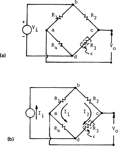
Example 3-14. For the bridge circuits in Fig. 3-38, assume that R₁ = R₂ = R₃ = R₄ = R and the bridge has one active gage R₃. (a) Find V_o when the bridge is driven by an ideal voltage source V_ι. (b) Repeat for the ideal current source I_i.

Solution: (a)  When R₃ becomes (R + ΔR) due to the applied strain, we obtain from Fig. 3-38a and Eq. 3-56

$\begin{array}{lll}\frac{V_o}{V_i}\hfill & =\hfill & \frac{R+\Delta R}{R+R+\Delta R}-\frac{R}{R+R}=\frac{\Delta R/R}{2\left(2+\Delta R/R\right)}\hfill \\ \hfill & =\hfill & \frac{\Delta R}{4R}\left[1-\frac{\Delta R}{2R}+{\left(\frac{\Delta R}{2R}\right)}^2-\cdots \right]\hfill \end{array}$

(3-66)

(b)  For the circuit in Fig. 3-38b, I₁ = I₂ when the bridge is balanced, and the output is V_o = 0. The output due to the strain applied to R₃ is

$V_o=R_3{I}_2-R_4{I}_1=\left(R+\Delta R\right)I_2-R_4{I}_1$

The currents I₁ and I₂ form a current divider for I_i. Thus

$\begin{array}{lll}\frac{I_2}{I_1}=\frac{R_1+R_4}{R_2+R_3}=\frac{2R}{2R+\Delta R}\hfill & \text{and}\hfill & I_1+I_2=I_{\text{ι}}\hfill \end{array}$

Eliminating I₁ and I₂ between the three equations above and simplifying, we get

$\frac{V_o}{I_{i}R}=\frac{\Delta R}{4R}\frac{1}{1+\Delta R/4R}=\frac{\Delta R}{4R}\left[1-\frac{\Delta R}{4R}+{\left(\frac{\Delta R}{4R}\right)}^2-···\right]$

(3-67)

Note that the output V_o for the constant-current drive in Fig. 3-38b is no longer linear with ΔR/R, as it was in Eq. 3-63. The nonlinearity in Eq. 3-66 for the constant-voltage drive is due to the term ΔR/2R, and that in Eq. 3-67 for the constant-current drive is due to ΔR/4R. Hence the constant-current drive is slightly more linear.

3-6.  SYSTEMS WITH FEEDBACK

Servomechanism and regulators are used extensively in instrumentation. The power steering of a car is a servo. The home thermostat is a regulator. The guidance and control of missiles and automation in industrial plants are examples of feedback. In view of the diverse applications, feedback is a general principle rather than the description hardware.

Feedback examines the structure of the arrangement of components in an instrument. The information model of single-input, single-output components will be used to describe the effect of feedback on the characteristics of components and the overall system performance. Stability analysis and design of feedback systems belong to another course.

A.  System Description

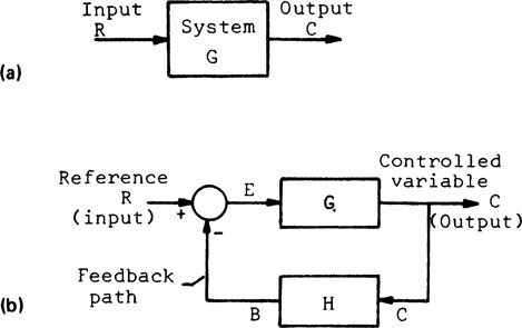
A system is either open loop or closed loop. An open-loop system is without feedback, as shown in Fig. 3-39a. The system equation is

FIGURE 3-39 Open loop and feedback systems. (a) Open-loop system. (b) Closed-loop system.

$C=GR$

(3-68)

where R is the input, C the output, and G the system transfer function.

The closed-loop system shown in Fig. 3-39b has a feedback path to complete the loop. The output C (controlled variable) is the input to the feedback element H. The feedback signal B from H is compared with the input R (reference) in a summer. The actuating signal E = (R – B) is applied to the feedforward element G (process) to produce the output C in order to complete the loop. The descriptions in equation form are

$\begin{array}{lll}C=GE\hfill & B=HC\hfill & E=R-B\hfill \end{array}$

(3-69)

Substituting the last two equations into the first and simplifying, we obtain the basic equation for feedback theory:

$\frac{\text{output}}{\text{input}}=\frac{C}{R}=\frac{G}{1+GH}$

(3-70)

Since E = R – B, the feedback is negative or degenerative. Only negative feedback systems are examined. Positive or regenerative feedback is seldom used except in complex systems.

The block diagram in Fig. 3-39b has only two types of symbols interconnected by signal flow paths. The symbols are the transfer function blocks G and H, and the summer that gives E = R – B. The summer is also called a differential or a comparator.

As an example, let the block diagram in Fig. 3-39b represent the position controller of a milling machine. C is the position of the turret of the machine, G the electric motor that turns the turret, and if a potentiometer that converts C to a voltage B. The turret is initially stationary and C = 0. A step input voltage R directs the turret to a reference position. The instantaneous voltage applied to the motor is E = R – B = R – HC = R – 0 = R. As the motor starts to turn, C deviates from zero and E = R – HC < R, that is, less voltage is applied to the motor. The motor stops when the turret reaches its final position as commanded by B, that is, when C is at the reference position, E = R – B = 0.

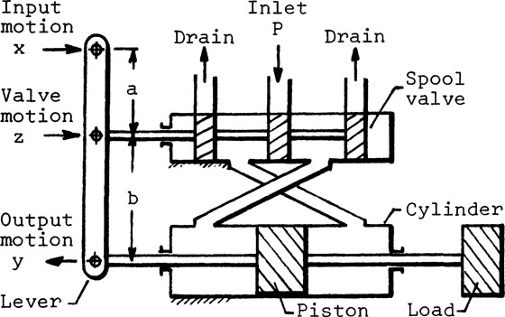
Example 3-15. The hydraulic position controller in Fig. 3-40 consists of an actuator (cylinder and piston), a spool valve, and a lever. The arrows indicate the positive directions for the displacements x, y, and z. If the piston is stationary and x is a step input, z opens the valve to admit high-pressure fluid to the cylinder. The piston then moves in the y direction, which is fedback through the lever to close the valve. The valve is closed when y is at the position commanded by x. Derive the system equation, assuming that the velocity of the piston is proportional to the valve opening.

FIGURE 3-40 Hydraulic position controller.

Solution: The equation for the motion of the lever is

$\begin{array}{lll}Y\hfill & =\hfill & f\left(X,Z\right)\hfill \\ \Delta Y\hfill & =\hfill & \begin{array}{lll}{\frac{\partial f}{\partial X}|}_{z=0}{\Delta X+\frac{\partial f}{\partial Z}|}_{x=0}\Delta Z\hfill & \text{or}\hfill & y=\frac{b}{a}x-\frac{a+b}{a}z\hfill \end{array}\hfill \end{array}$

where X, Y, and Z are the total displacements, and x, y, and z their incremental values. The motion of the piston is given as

$\frac{dy}{dt}=Cz$

where C is constant. Eliminating z from the equations gives

$\begin{array}{lll}\frac{a+b}{aC}\frac{dy}{dt}+y=\frac{b}{a}x\hfill & \text{or}\hfill & \text{τ}\frac{dy}{dt}+y\hfill \end{array}=Kx$

(3-71)

where τ is the time constant and K the sensitivity of the controller. The equation shows that the steady-state response is y = Kx; that is, the position y is proportional to the command x.

Feedback has many advantages. As a null balance system, it is capable of high accuracy. The feedback enables the system to perform a task automatically and to be self-correcting. For the example above, if the output C exceeds the position commanded by R, the feedback returns C to the desired position in order to achieve E = 0. It will be shown that feedback can be used to modify the characteristics of components as well as to enhance the dynamic performance of a system. Finally, a computer can be a part of the control loop in a complex system. The system can be adaptive to the environment to yield an optimum performance.

Feedback is not without disadvantages. It adds complexity, and the system can be unstable. As a null balance transducer, it is inherently slower than the unbalance type (see Sec. 3-2).

B.  Effects on Characteristics of Components

Characteristics of components in a measuring system may change due to environmental conditions or the deterioration of parts. In this section we show that the characteristics can be stabilized by means of feedback.

Consider the deterioration of G in the open-loop system shown in Fig. 3-39a. From Eq. 3-68 the effect of G on the output C is

$\frac{dC}{C}=\frac{dG}{G}$

This states that for a given R, the change in the output C is proportional to the change in G. If G is a control valve, a 10% change in its characteristic will cause a 10% change in the flow.

Now, examine the effect of G on the output C in a feedback system. Assume that R and H remain constant. Differentiating Eq. 3-70 with respect to G yields

$\frac{dC}{R}=\frac{dG}{1+GH}-\frac{GHdG}{{\left(1+GH\right)}^2}=\frac{dG}{{\left(1+GH\right)}^2}$

Multiplying the left side by R/C and the right side by (1 + GH)/G and assuming that GH ≫ 1, we obtain

$\frac{dC}{C}=\frac{1}{1+GH}\frac{dG}{G}\simeq \frac{1}{GH}\frac{dG}{G}$

(3-72)

For example, if GH = 100, a 10% change in G will result in a 0.1% change in the output C. Hence the performance of a system with feedback is insensitive to the changes in G.

The feedback, however, will not compensate for the changes in H. Assume that R and G remain constant. Differentiating Eq. 3-70 with respect to H yields

$\frac{dC}{C}=-\frac{GdH}{1+GH}\simeq -\frac{dH}{H}$

(3-73)

Let us examine the implications of feedback from Eqs. 3-72 and 3-73. G is the process under control. It is at a high power level involving large components. H deals with the feedback signal at a low power level. H has small-size components usually with passive components. Hence H can be made accurate rather inexpensively. Moreover, H can be stabilized with its own feedback loop. The deductions from Eqs. 3-72 and 3-73 are correct, but the feedback enables the control of G more precisely and economically.

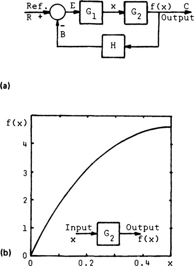
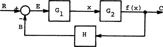
Example 3-16. The feedback system in Fig. 3-41a has G = 10, and H = 0.1. G is nonlinear as shown in Fig. 3-41b. Plot the overall characteristics of C versus R for 0 < R < 0.5 to show that the feedback has a linearizing effect [18].

Solution: From Fig. 3-41a, we get

$\begin{array}{lll}C\hfill & =\hfill & f\left(x\right)\hfill \\ x\hfill & =\hfill & G_{1}E=G_1\left(R-HC\right)=G_{1}R-G_{1}HC\hfill \end{array}$

(3-74)

The last equation is rearranged to give a straight line

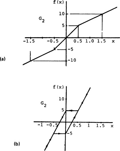
FIGURE 3-41 Reducing nonlinearity with feedback. (a) Feedback system. (b) Characteristic of G₂.

$C=-\underset{\text{slope}}{\underbrace{\frac{1}{G_{1}H}}}x+\underset{\text{constant}}{\frac{R}{H}}$

(3-75)

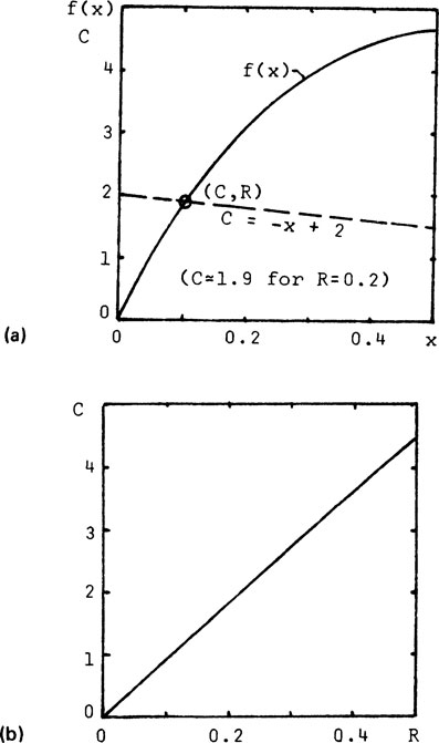
The characteristic for C versus R is found graphically from the simultaneous solution of Eqs. 3-74 and 3-75 for 0 < R < 0.5. Equation 3-74 is replotted in Fig. 3-42a. Assuming a value of R, Eq. 3-75 gives a straight line. For example, if R = 0.2, we get

$C=-\frac{1}{10\times 0.1}x+\frac{0.2}{0.1}=-x+2$

FIGURE 3-42 Reducing nonlinearity with feedback. (a) Graphical construction. (b) C versus R with feedback.

This is shown as a dashed line in Fig. 3-42a. The lines intersect at (C,R) = (1.9,0.2). The process is repeated for the range of values of R. The resulting characteristic for C versus R in Fig. 3-42b shows that the nonlinearity of G is minimized by means of feedback.

C.  Effects on System Performance

In this section we generalize the effects of feedback presented in the preceding section. An ac amplifier (see Sec. 3-3D) with feedback is used to illustrate the discussions [19].

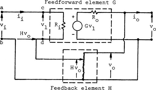
The model of an ac amplifier with voltage feedback is shown in Fig. 3-43. The feedforward element is a unilateral controlled-source device, with an input impedance R_ι, an output impedance R_o, and a controlled voltage source Gυ₁, where G = υ_o/υ₁ is the transfer function for the open-circuit voltage gain without feedback. The feedback element H is a potentiometer with a feedback voltage Hυ₀ for 0 < H < 1.

For the amplifier with negative feedback, the input loop gives

${\upsilon }_1={\upsilon }_i-H{\upsilon }_o$

(3-76)

This corresponds to E = R – B in Fig. 3-39. From G = υ_o/υ₁ and Eq. 3-76, we obtain

$\begin{array}{lll}{\upsilon }_O=G{\upsilon }_1=G\left({\upsilon }_1-H{\upsilon }_0\right)\hfill & \text{or}\hfill & \frac{{\upsilon }_0}{{\upsilon }_{\text{ι}}}=\frac{G}{1+GH}=G_f\hfill \end{array}$

(3-77)

FIGURE 3-43 Amplifier with voltage feedback.

where G_f is the overall voltage gain with feedback and the subscript f denotes the feedback. Note that Eq. 3-77 is identical to Eq. 3-70 for the basic feedback system.

Case 1. Improving Dynamic Response

If the gain G in Eq. 3-77 is very large, such that GH ≫ 1, and H, a constant, the overall gain G_f in Eq. 3-77 reduces to

$\begin{array}{lll}{G}_f=\frac{1}{H}\hfill & \text{for}\hfill & GH\gg 1\hfill \end{array}$

(3-78)

This states that the gain G_f for an amplifier with feedback is constant independent of the operating frequency, from zero to infinity. In reality, the gain G for the amplifier without feedback is not constant, and GH ≫ 1 cannot be maintained for all frequencies. The implication, however, is that degenerative feedback will improve the overall dynamic response.

Case 2. Increasing input and Decreasing Output impedance

The input impedance for the amplifier without feedback, as measured across the terminals c and d in Fig. 3-43, is R_i.

${\upsilon }_1=R_i{i}_{\text{ι}}$

The input impedance with feedback, as measured across the terminals a and b, is R_fi.

${\upsilon }_i=R_{f\iota }{i}_{\iota }$

Hence the ratio of the impedances is

$\frac{R_{fi}}{R_i}=\frac{{\upsilon }_i}{{\upsilon }_1}$

Eliminating υ_o between Eqs. 3-76 and 3-77 gives

${\upsilon }_i=\left(1+GH\right){\upsilon }_1$

(3-79)

Substituting υ_i/υ₁ from the equations above, we get

$R_{fi}=\left(1+GH\right)R_i$

(3-80)

If GH ≫ 1, the input impedance of the amplifier with feedback is increased by a factor of (1 + GH).

From Fig. 3-43 the output impedance of the amplifier without feedback is R_o. Let us use the Thevenin’s equivalent in Fig. 3-11 to illustrate the measurement of R_o. From V = RI, where V = V_eq = Gυ₁ = V_oc (open circuit), R = R_o, and I = I_sc (short circuit), we obtain

$\begin{array}{lll}{V}_{oc}=R_o{I}_{\text{sc}}\hfill & \text{or}\hfill & R_o=\frac{V_{\text{oc}}}{I_{\text{sc}}}\hfill \end{array}$

Similarly, the output impedance R_fo of the amplifier with feedback in Fig. 3-43 is defines as

$R_{fo}={\upsilon }_o/{\left(i_o\right)}_{\text{sc}}$

(3-81)

where υ_o is the open-circuit voltage with feedback from Eq. 3-77.

$\frac{{\upsilon }_o}{{\upsilon }_i}=\frac{G}{1+GH}$

When the output of the amplifier in Fig. 3-43 is short circuited, the loop equation is

$G{V}_1=R_o{\left(i_o\right)}_{\text{sc}}$

(3-82)

Furthermore, when the output is shorted, there is no feedback signal and υ₁ = υ_i. Substituting υ_o and (i_o)_sc into Eq. 3-81 and noting that υ₁ = υ_i, we obtain

$R_{fo}=\frac{1}{\left(1+GH\right)}{R}_o$

(3-83)

Hence the output impedance R_fo with feedback is less than R_o without feedback by a factor of (1 + GH).

Case 3. Reducing Distortion

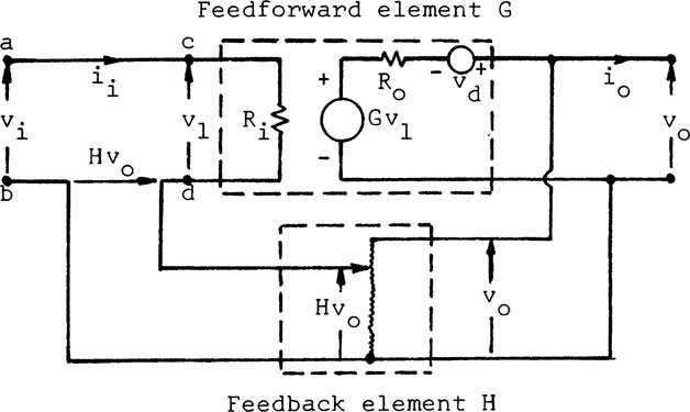
Assume the amplifier in Fig. 3-44 has a distortion voltage υ_d. The voltage output without feedback is

${\upsilon }_o=G{\upsilon }_1+{\upsilon }_d$

(3-84)

The feedback signal is

$H{\upsilon }_o=H\left(G{\upsilon }_1+{\upsilon }_d\right)$

(3-85)

Substituting Hυ_o into Eq. 3-76 and simplifying, we get

$\left(1+GH\right){\upsilon }_1={\upsilon }_1-H{\upsilon }_d$

Eliminating υ₁ between Eq. 3-84 and the equation above and rearranging, we obtain

${\upsilon }_o=\frac{G}{1+GH}{\upsilon }_{\text{ι}}+\frac{1}{1+GH}{\upsilon }_d$

(3-86)

Hence the distortion voltage υ_d in the amplifier without feedback is reduced by a factor of (1 + GH) by means of feedback.

FIGURE 3-44 Use feedback to reduce distortions.

In summary, for all the examples presented, it is advantageous to use a high gain for G in order to have a large value for GH. Thus the performances can be improved by a factor of (1 + GH). Since components in a system will deteriorate with time, the technique presented is often used for stabilizing instruments.

3-7.  METHODS OF NOISE REDUCTION

Noise in a measurement may be from the undesired external inputs (see Eq. 2-4) or generated internally. Signal and noise are like quantities and they may or may not possess distinct characteristics. Methods of noise reduction for analog signals are examined in this section.

Had it not been for noise, instrumentation would be simple and straightforward. Once an experimental physicist was frustrated in an investigation of the slippage between crystals in metals. The amplification of an extremely weak signal was simple. Two operational amplifiers in cascade would amplify a million times or more. The noise, however, was amplified with the signal. It was the noise that “killed” the experiment.

A.  Noise Reduction at the Interface

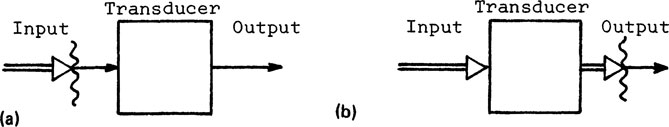
External noise inputs can be reduced at the input interface or the output interface of an instrument, as shown in Fig. 3-45. The double arrows denote the multiple quantities and the vertical wavy lines the interface for the noise reduction. Schemes commonly used for noise reduction are filtering and shielding.

FIGURE 3-45 Noise reduction at input/output interface. (a) Reduction at input. (b) Reduction at output.

Whenever possible, corrective measures should be applied at the input interface rather than at the output. First, the input is at a low power level and is more susceptible to noise pickups. A noise of constant magnitude will degrade the low-level signal at the input more than the higher-level signal at the output. Second, when the signal/noise ratio is low, the noise can saturate the instrument and produce extraneous signals at the output (see Sec. 2-2D). Finally, even when the signal/noise ratio is high, the noise could be at a resonant frequency of the instrument and produce undesired effects, such as in the tool dynanometer described in Sec. 1-3A.

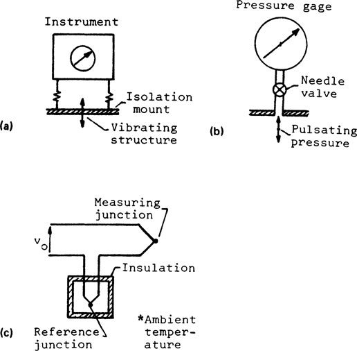
Isolation implies the separation of the instrument from a hostile environment and is often called a noise reduction technique. Isolation, however, is only loosely defined. The isolation mount in Fig. 3-46a separates an instrument from the high-frequency vibration at its base by means of soft springs. Thus the isolation mount is a frequency-selective filter. Another example is a pressure gage with a needle valve, shown in Fig. 3-46b. The gage will indicate slow pressure changes in a tank but will not respond to the high-frequency pulsating pressure of the air compressor. The thermocouple in Fig. 3-46c isolates the reference junction from the ambient temperature by means of a thermal shield. An isolation transformer is often used to eliminate the effect of ground loops in instruments. The effective use of isolation transformers requires a good knowledge of electrical shielding [20]. Since isolation is only loosely defined, we shall not belabor the subject.

1.  Filters

When the signal and noise possess distinct characteristics, a filter can be used to separate the signal from the noise by means of selective filtering. For example, the air filter in a home furnace is size selective. A light filter for photography is frequency selective according to the wavelengths of light. Isotopes of chemical elements have identical chemical properties, but they can be separated mechanically by means of a centrifuge. The suspension system of an automobile is an example of frequency-selective filtering. It filters out the high-frequency road roughness to give passengers a smooth ride.

FIGURE 3-46 Examples of noise reduction. (a) Vibration isolation. (b) Throttling. (c) Thermal isolation.

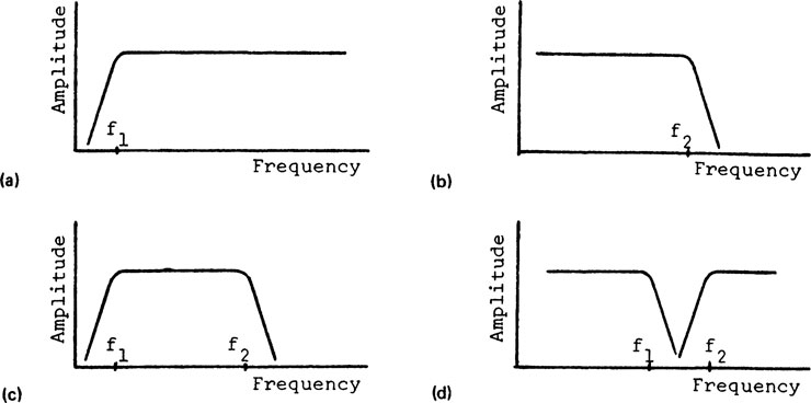
Electrical filters for instruments are frequency selective. They are classified as high-pass, low-pass, bandpass, and band-reject. Simple filters can be constructed from resistors and capacitors. This is described in Chapter 4. Design formulas for passive filters are found in the literature [21].

A high-pass filter passes the high-frequency components of an input signal and rejects the low-frequency components below the cutoff frequency f₁ as shown in Fig. 3-47a. The cutoff is not abrupt. The sharpness of the filter is described by the slope at cutoff. Active electronic filters with a slope of 16:1 or higher are common.

A low-pass filter passes the low-frequency components of an input signal and rejects the high-frequency components above the cutoff frequency f₂, as shown in Fig. 4-37b. It is interesting to note that mechanical systems are inherently low-pass filters. Due to the inherent mass, a mechanical system does not respond to extreme high frequencies. This observation may serve to explain certain test results or can be capitalized in applications.

FIGURE 3-47 Characteristics of filters. (a) High-pass. (b) Low-pass. (c) Bandpass. (d) Band reject.

A series combination of a high-pass and a low-pass filter gives a bandpass filter. A broadband filter passes the harmonic components of its input signal from frequency f₁ to f₂, as shown in Fig. 4-37c. For example, the audio-frequency range is from 20 Hz to 20 kHz. A narrowband filter, with a bandwidth of a few hertz in the range of kilohertz, is often used for the detailed examination of the harmonic contents in a signal, such as in a vibration test. In this case, f₁ is very close to f₂ and the filter characteristic appers as a spike.

A parallel combination of the high-pass and low-pass filters gives a band-reject filter, as shown in Fig. 3-47d. The filter rejects the harmonics in the input signal within the frequency band between f₁ and f₂. This filter can be used in a recorder to prevent the 60-Hz noise voltage from saturating its amplifier.

Statistical filtering or signal averaging is used when the signal and noise occupy the same part of the frequency spectrum, but the signal is repetitive and the noise random. The method synchronizes the data sampling with the repetitive signal. If a large number of data samples are averaged, the random noise will average to zero, while the repetitive signal will converge to its mean value. The technique is also useful for low signal/noise ratio signals. This filtering technique can be done by analog or digital means.

2.  Shields

Shielding blocks the noise inputs from a measuring system, while filtering separates the noise from the signal. Hence a shield is directed toward the noise source, while a filter is directed toward both the signal and noise. Shielding for noise reduction should be built into a system. In this section we describe the shielding of electrical fields and magnetic fields.

A noise voltage due to an electric field can loosely be called the antenna effect. For example, an oscilloscope will show a large 60-Hz noise pickup when an unshielded cable is connected to its input. The noise level increases when the lead is touched with a bare hand, particularly when the hand is moist. The person touching the signal lead has extended the antenna.

A shielded cable is shown in Fig. 3-48. The signal lead is shielded when the shield in the form of a braided copper mesh is connected to ground. The shield minimizes the voltage pickup between the signal lead and the surrounding electric field. This is called an electrostatic shield. First, the shield intercepts the surrounding electric field and a voltage is induced in the shield due to the antenna effect. The voltage in the shield will also induce a voltage in the signal lead by virtue of the distributed capacitance between the shield and the lead. Second, the ground connection drains the charge in the shield to ground to render the shield at the ground potential. Hence the signal lead of a shielded cable is free of the surrounding electric field. An instrument is shielded in like manner by means of a metallic chassis.

A ground is the common connection. An earth ground is analogous to the sea level for the measurement of elevation. A chassis ground or a floating ground is simply a common connection in an instrument, and it is not connected to earth. A ground is analogous to a sump in a hydraulic network. Not all sumps are at the same level.

FIGURE 3-48 Shielded cable for electric field.

Similarly, not all grounds in a measuring system are at the same potential. Even the grounds of electrical outlets in the same laboratory may have a potential differential. When a system has two grounds at different potentials, a current will flow from one ground to the other, thereby forcing a part of the system to complete the circuit. This is called a ground loop. By analogy, a flow will occur in a hydraulic network when two sumps of different potential are connected. A current flow in the signal lead due to the ground loop is equivalent to a voltage signal. For example, a 10-μA current in a 2-Ω line will appear as a 20-μV signal. When noise occurs in a low-level signal lead, it will be amplified together with the signal. Hence all signal grounds, shield grounds, and power grounds in a measuring system should be tied to only one common ground. By the same token, a shield should be ground at only one point.

The requirements for an electrostatic shield are a high degree of coverage of the low-level signal portion of an instrument, and a shield of high conductive material, such as copper. General rules for shielding and grounding are stated by Morrison [22].

A noise voltage from a magnetic field is due to the generator effect. For example, a voltage is induced in a conductor moving in a magnetic field, such as a vibrating signal lead or a strain gage in a shock test. Alternatively, a voltage is induced in a stationary signal lead in a changing magnetic field from a motor or a transformer. A magnetic noise pickup can be from a rotating machine part, the magnetic flux of which is from the magnetization in past inspection.

Magnetic shielding is achieved by minimizing the coupling between the magnetic flux and the instrument.

1.  A first choice for reducing the coupling is by menas of a physical separation, since the field strength is inversely proportional to the distance squared.

2.  The magnetic coupling can be reduced by avoiding loops in the signal leads or by a reorientation of the leads. It may be possible to divert the flux away from the instrument by providing an alternative path for the flux.

3.  A shield can be used to attenuate the magnetic flux entering the intended shielded area. The shielding material must have a high magnetic permeability, such as a ferromagnetic material. A large amount of shielding material is generally required compared with electrostatic shielding.

In summary, electrostatic shields are more common than magnetic shields in instrumentation. Electric and magnetic fields are separate mechanisms and different criteria are required for their shielding. An electrostatic shield will not serve as a magnetic shield, and a magnetic shield in general is not a good electric shield. It is best to avoid a magnetic field than to attempt a shielding.

B.  Noise Reduction by Insensitivity

Noise reduction by decreasing the sensitivity of instruments for the undesired inputs is discussed in this section (see Sec. 2-1A). The techniques presented are inherent insensitivity, cancellation, and information conversion.

1.  Inherent Insensitivity

Physical laws for sensing were described in Sec. 2-1. The signal and noise component for the first-order effects are shown in Eq. 3-87 (see Eq. 2-5).

$\underset{\text{output}}{\underset{\nearrow }{\Delta Y}}=\underset{\text{signal}}{\underbrace{\frac{\partial f}{\partial D}|{}_0\Delta D}}+\underset{\text{noise}}{\underbrace{\frac{\partial f}{\partial U}|{}_0\Delta U}}$

(3-87)

where D is the desired input and U all the undesired inputs. The system is inherently insensitive to the noise inputs when ∂f/∂U = 0. This is achieved by (1) the proper selection of material and/or operating conditions, or (2) a structural change in the system, such as feedback. The discussions presented previously will not be repeated here.

The selection of material and operating conditions should be considered together for the given application. Consider the operation conditions for ∂f/∂U = 0 in a strain measurement, where U is the undesired temperature input. A strain gage made of constantan is temperature insensitive for the operating temperature at 75°F for the range 50 to 100°F, as shown in Fig. 3-49. It is also insensitive to temperature if when operating at 275°F for the range 250 to 300°F. As stated in Sec. 2-1, the conditions ∂f/∂U = 0 is necessary only for the given range of operation.

Now, consider the selection of material for an application. The strain gage of the isoelastic material is more temperature sensitive, but it also has a higher gage factor and therefore greater sensitivity [24]. For dynamic measurements and over a relatively short period, the isoelastic gage may be more suitable than the constantan gage, particularly when the test setup has a long time constant. In other words, an undesired effect can be ignored if it does not interfere with the given application.

An example of inherent insensitivity by means of a structural change in a strain measurement is shown in Fig. 3-50, in which a non-noise generating component is substituted for a noise-generating component. Signal from the strain gage on a rotating shaft is brought out by means of a pair of slip rings. A slip ring is a metallic ring on a shaft to transfer the signal from a rotating member to the stationary instrument. The ring is insulated from the shaft. A ballast circuit is used for the measurement, as shown in Fig. 3-50b. The circuit is unsatisfactory because of the unpredictable contact resistance at the brushes. The signal can be completely masked by the brush noise (see Prob. 1-4).

FIGURE 3-49 Typical apparent strain for two alloys commonly used in strain gages. (From Ref. 23.)

FIGURE 3-50 Noise reduction by insensitive structure. (a) Signal from rotating shaft. (b) Ideal voltage source V_i (c) Ideal current source I_i. (From Ref. 25.)

The problem is solved by replacing the voltage source with a current source I and using two pairs of slip rings instead of one pair, as shown in Fig. 3-50c. Since I is constant, the contact resistance at the slip rings has no effect on the current flow. Since υ_o is measured with a high-impedance voltmeter, there is no current flow in the voltage measurement and the brush noise has no effect on the signal transmission.

2.  Cancellation

The differential method is used for noise reduction by cancellation. Assume two identical sensors A and B. When A and B are exposed to an undesired environment, they can be arrange for noise cancellation by means of opposing effects (1). When A is exposed to the environment and B only to the undesired inputs, A and B can be arranged for noise cancellation by means of equal effects due to the undesired inputs (2).

Noise cancellation by opposing effects is commonly used in instrumentation for transducers exposed to the same environment. For example, signal leads are often in twisted pairs to cancel the noise pickup in a measurement. When a magnetic field is undesired in a strain measurement, two strain gages can be made noninductive by means of a side-by-side mounting, as shown in Fig. 3-51a. The magnetic field produces equal effects in the gages, but the gages are mounted in series opposition to cancel the effect. In practice, identical transducers are not necessary for cancellation by opposing effects. For example, a transistor with a negative temperature coefficient can be used to compensate for the temperature effect on an electronic circuit with a positive temperature coefficient.

Noise cancellation by equal effects in a pressure measurement is shown in Fig. 3-51b. Transducers A and B are exposed to the same undesired effects, such as shock and temperature, but A is subjected to the pressure input and B is vented to the atmosphere. The differential output A – B gives the desired output relative to atmospheric pressure.

Similarly, the adjacent strain gages A and B in Fig. 3-52a are exposed to the same environment, but only A is subjected to the strain input. Gage B is the “dummy” gage for temperature compensation. The differential output gives the strain signal. The resistances in the lead wires must also be compensated. The leads are of the same length and exposed to the same environment. The effects of the leads will cancel if they are on adjacent arms of the bridge circuit. The three-wire system has the advantage that there is no current in the center lead when the bridge is balanced. The four-wire system provides greater flexibility when using two sensors.

3.  Information Conversion

Information conversion changes the characteristics of the signal without altering its information content (see Sec. 2-3). The input signal modulates the carrier to produce a modulated output, which is at a higher power level as well as less susceptible to noise. Modulation is treated in Chapter 5. Mechanical modulation in an optical pyrometer is described to illustrate the process [26],

FIGURE 3-51 Noise reduction by cancellation. (a) Noninductive resistance wire sensors. (b) Pressure transducers.

The optical pyrometer in Fig. 3-53a, used for measuring the temperature T from a source, can be made inherently insensitive to the ambient temperature T_a. Assume that the waveforms of T and T_a are as shown in Fig. 3-53b and Fig. 3-53c, respectively. If the output of the pyrometer is proportional to T + T_a, the signal T can be masked by the noise T_a.

FIGURE 3-52 Compensation for resistance in leads. (a) Four-wire system. (b) Three-wire system.

The chopper in the pyrometer converts T into a high-frequency ac signal T_c. The chopper is a slotted disk and acts as a mechanical shutter. Thus the output of the sensor υ₁ is the proportional to T_c + T_a, as shown in Fig. 3-53d. Since T_a is slowly varying, its frequency is below the cutoff frequency of the ac amplifier, and T_a is rejected by the amplifier. Hence the amplifier output υ₂ is shown in Fig. 3-53e. The original signal T is shown as a dashed line in the figure. It can be recovered from υ₂ by means of a demodulation process.

3-8.  NOISE DOCUMENTATION

The method for noise documentation is similar to that for calibration described in Sec. 2-4. The principle of calibration is that a known input produces a known output, and a zero input produces a zero output. An output without a corresponding input is noise in the system. When the noise level is identified and the measuring system calibrated for in-service conditions, the experimenter can vouch for the validity and accuracy of the data. A method for noise documentation by Stein is described in this section [27].

The steps for the documentation are: (1) systematically identify the information paths in a measurement, and (2) sequentially reduce the noise from each path to the residual level. The noise levels for each signal path are thus documented.

The general model for transducers (see Fig. 2-17) is used for this discussion. The information paths 1 to 4 are identified in the model in Fig. 3-54a. The strain gage bridge in Fig. 3-54b is used to illustrate the process. The switches 1,2, and 3 are added for the purpose of noise documentation and circuit calibration. The switches are shown in the normal operating positions. Since the switches can be operated before, during, and after a run, the noise level can also be documented before, during, and after a run.

It should be reiterated that the noise for each step should be reduced to a residual level and documented before the next step is executed.

Step 1: Component check. Close switch 3 to position d. This preliminary step checks the noise in the components downstream from the transducer. Since the input to the components is shorted, the output υ_o should be zero. If not, the noise in the components should be reduced to a residual level before the execution of the next step.

Step 2: Information path 1. Switch 1 to position a. Switches 2 and 3 at normal positions. Measurand OFF; that is, no strain is applied to the gages. Since the measurand and the carrier voltage V are off, there is no non-self-generating signal. From Fig. 3-54a the output υ_o must be from the self-generating part of the system. This is the noise from the undesired inputs in path 1.

FIGURE 3-53 Noise reduction by information conversion. (a) Schematic of optical pyrometer, (b) Source temperature. (c) Ambient temperature. (d) Sensor output. (e) Amplifier output.

Step 3: Information paths 1 and 2. Measurand OFF. All switches in their normal positions. Since the measurand is off, the output υ_o must be from paths 1 and 2, as shown in Fig. 3-54a. The noise is from the self-and non-self-generating parts of the undesired input.

Step 4: Information paths 1 and 3. Switch 1 at a. Switches 2 and 3 at normal positions. Measurand ON. Since the carrier V is OFF, the output υ_o can only be from the self-generating part of the transducer. Thus the residual noise in paths 1 and 3 are documented.

Step 5: All paths. Measurand ON. All switches in normal positions. The output υ_o is due to the measurand and all the residual noise in the previous steps. Thus the signal/noise ratio can be found and the amount of noise in the output is known.

FIGURE 3-54 Transducer model and method for noise documentation. (a) Model of transducer and information channels. (b) Checking information channels.

PROBLEMS

  3-1.  With the aid of a sketch when necessary, briefly discuss each of the following:

(a) Differential measurement.

(b) Comparative measurements.

(c) Comparison of methods of measurement.

(d) One-, two-, and three-port devices.

(e) Basic circuits for non-self-generating transducers.

(f) Using feedback for correcting nonlinearities.

(g) Filtering and shielding.

(h) Methods for noise reduction.

  3-2.  A force transducer of stiffness k_m is inserted as shown in Fig. P3-1 for measuring the static force transmitted through k₁. Find the ratio force_measured/force_true in the measurement.

  3-3.  A displacement gage of stiffness k_m is placed as shown in Fig. P3-2 for measuring the static deflection of the mass m. Find the ratio x_measured/x_true in the measurement.

  3-4.  Find the ratio force_measured/force_true for the static force in k₂ by means of a force transducer of stiffness k_m, as shown in Fig. P3-3.

  3-5.  The characteristic of a transducer is Y = 2X² for X > 0, and Y = 0 for X ≤ 0. Two transducers are used in a differential measurement. (a) If the neutral position is at X₀ = 0.3, derive an expression for the output, (b) Show a plot of the output for X₀ = 0.3 and ΔX = ±0.3.

  3-6.  Repeat Prob. 3-3 if Y = 2e^x for X > 0, and Y = 0 for X < 0. (a) Assume that X₀ = 1.0 and ΔX = ±0.5. Find the deviation from linearity, (b) Repeat for X₀ = 2 and ΔX = ±0.5.

  3-7.  The strain gage bridge in Fig. P3-4 is used as a differential transducer. Initially, R₁ = R₂ = R₃ = R₄ = R. (a) Find the output voltage V_o if the bridge uses four active gages, (b) Repeat part (a) (1) if R₁ and R₂ are active, (2) if R₂ and R₃ are active, and (3), if only R₃ is active.

  3-8.  The output voltage of the strain gage bridge in Fig. P3-5 is measured by means of a galvanonometer of resistance R_m = 100 Ω. Initially, R₁ = R₂ = R₃ = R₄ = 120 Ω. Assume that G_f = 2.0, V_i = 5 V, and ΔR/R = 0.001 for each of the four gages due to the applied strain. (a) Find the voltage across R_m. (b) Find the deflection of the galvanometer if its sensitivity is 0.1 μA/mm.

  3-9.  The strain gage bridge in Fig. P3-6 is calibrated by means of R_c. Assume that R₁ = R₂ = R₃ = R₄ = 120 Ω, G_f = 2.0, and V_o reads 150 units for the calibration, (a) Find the equivalent strain applied to R₂ in the calibration, (b) If the bridge uses two active gages for a measurement and V_o = 500 units, what is the applied strain? (c) If all four gages of the bridge are active and V_o = 500 units, what is the applied strain? (d) Propose a scheme for using four active gages in a tensile test. If V_o reads 500 units, what is the axial tensile strain?

3-10.  An air gage is used for measuring the displacement x of the flapper valve in Fig. P3-7. Assume that the flow rate Q is

$Q=f\left(P_0,P_1,d_1,d_2,x\right)$

where P’s are gage pressures and P₀ = constant, (a) Derive an expression for P₁/P₀ in terms of d₁, d₂, and x. (b) Find the maximum sensitivity of the gage, (c) If d₁ = d₂ = 0.02 in., P₀ = 10 in. of water, and P₁ can be read to 0.1 in. of water, find x_min that can be detected, (d) Plot P₁/P₀ versus $d_{2}x/d_1^2$ for $0<d_{2}x/d_1^2<1$. (e) Plot sensitivity versus $d_{2}x/d_1^2$ for $0<d_{2}x/d_1^2<1$.

3-11.  Draw the sketch of a differential transducer, using two of the air gages shown in Fig. P3-7. P₁ of gage 1 measures x₁ = x₀ ∓ Δx and P₂ of gage 2 measures x₂ = x₀ ∓ Δx. (a) Using the data in Prob. 3-10 and assuming that the neutral position of the flapper valve is x₀ = 0.01 in. of water, plot (P₁ – P₂)/P₀ versus Δx for −0.01 < Δx < 0.01. (b) Find the sensitivity of the differential gage at x₀ = 0.01 in. of water.

3-12.  An ac amplifier circuit and the static characteristics of its transistor are shown in Fig. P3-8. (a) Determine the operating point Q of the amplifier. (b) Given h_ie = 3.6 kΩ, h_re = 3 × 10⁻³, h_fe = 150, and h_oe = 1.4 × 10⁻⁴S. Calculate the voltage and current gain and the input and output impedance of the amplifier.

3-13.  (a) Draw the ac equivalent circuit for the transistor amplifier shown in Fig. P3-9. (b) Derive an expression for the voltage gain υ_o/υ_i. (c) Given R₁ = 930 kΩ, R₂ = 250 kΩ, R_E = 3 kΩ, h_re = 3.6 kΩ, h_fe = 3 × 10⁻³, h_fe = 150, and h_oe = 1.4 × 10⁻⁴ S. Find the voltage gain and the input impedance of the amplifier.

3-14.  A two-stage amplifier is shown in Fig. P3-10. The first stage is represented by its Thévenin’s equivalent. For the transistor of the second stage, assume that h_ie = 2 kΩ, h_re = 0.001, h_fe = 70, and h_oe = 50 μS. Derive the ac equivalent circuit and an expression of the overall voltage gain.

3-15.  A feedback system with a nonlinear component G₂ is shown in Fig. P3-11. G₁ = 10, H = 0.1, and the characteristics of G₂ is

Plot the overall characteristics of C versus R for 0 ≤ R ≤ 1.0.

3-16.  Repeat Prob. 3-15 for the characteristics of G₂ shown in Fig. P3-12a.

3-17.  Repeat Prob. 3-15 for the characteristics of G₂ shown in Fig. P3-12b.

3-18.  Referring to Fig. P3-15, the characteristics of G₂ is

$f\left(x\right)=20x-\frac{x^3}{2}$

Design the feedback system and specify the values of G₁ and H such that dC/dR = 20 for −2.5 < R < 2.5.

3-19.  Repeat Prob. 3-18 for dC/dR = 10 for −5 < R < 5.

FIGURE P3-1

FIGURE P3-2

FIGURE P3-3

FIGURE P3-4

FIGURE P3-5

FIGURE P3-6

FIGURE P3-7

FIGURE P3-8

FIGURE P3-9

FIGURE P3-10

FIGURE P3-11

REFERENCES

1.  Brophy, J., Basic Electronics for Scientists, 2nd ed., McGraw-Hill Book Company, New York, 1972, p. 228.

2.  ASTM Standards on Petroleum Products, Method D8, American Society for Testing and Materials, Philadelphia.

3.  Schlesinger, G., Testing Machining Tools, 8th ed., revised by F. Koenig-sherger and H. Burdenkin, Pergamon Press, Inc., Elmsford, N. Y., 1978.

4.  Stone, B. J., The Development of Dynamic Performance Tests for Lathes, Proceedings of the Twelveth International Machine Tool Design and Research Conference, Manchester, England, Sept. 1971, F. Koenigsberger and T. Tobias (eds.), Macmillan Publishing Company, New York, 1972, pp. 299–314.

5.  Ramboz, D. J., Self-Contained Electronic Vibration Meters and Special Purpose Transducers, in Shock and Vibration Handbook, 2nd ed., C. M. Harris and C. E. Crede (eds.), McGraw-Hill Book Company, New York, 1976, Chap. 14.

6.  Dranetz, A. I., and A. W. Orlacchio, Piezo-electric and Piezo-resistive Pickups, in Shock and Vibration Handbook, 2nd ed., C. M. Harris and C. E. Crede (eds.), McGraw-Hill Book Company, New York, 1976, Sec. 16.

7.  Stein, P. K. Measuring System Performance Capabilities as Governed by Input Conditions Design., Proceedings of Western Regional Strain Gage Committee Meeting, Sept. 21, 1970, Society of Experimental Analysis, Westport, Conn.

8.  Tse, F., I. Morse, and R. Hinkle, Mechanical Vibrations, 2nd ed., Allyn and Bacon, Inc., Boston, 1978, p. 48.

9.  Flanagan, P. M., Design of a Clinical Phono-angiography System, Ph.D. dissertation, University of Cincinnati, 1980.

10.  Tse, Morse, and Hinkle, Ref. 8, p. 176.

11.  Pipes, L. A., Matrix Methods for Engineers, Prentice-Hall, Inc., Englewood Cliffs, N. J., 1963, Chap. 12.

12.  Lynch, W. A., and J. G. Truxal, Signal and Systems in Electrical Engineering, McGraw-Hill Book Company, New York, 1962, Chap. 9.
Brown, P. B., G. N. Franz, and H. Moraff, Electronics for Modern Scientists, Elsevier Science Publishing Co., Inc., New York, 1982, Chap. 2.

13.  Cowles, L. G., Transistor Circuits and Applications, 2nd ed., Prentice-Hall, Inc., Englewood Cliffs, N. J., 1974, p. 11.

14.  Horowitz, P., and W. Hill, The Art of Electronics, Cambridge University Press, New York, 1980, pp. 650–652.

15.  Amey, W. G., et al., Bridges and Potentiometers, in Process Instruments and Control Handbook, 2nd ed., D. M. Considine (ed.), McGraw-Hill Book Company, New York, 1974, Sec. 14.

16.  Stein, P. K., The Constant Current Concept for Dynamic Strain Measurement, Strain Gage Read., Vol. 6, No. 3 (Aug.–Sept. 1963), pp. 53–72.

17.  Perry C. C., and H. R. Lissner, The Strain Gage Primer, 2nd ed., McGraw-Hill Book Company, New York, 1962, p. 93.

18.  West, J. C., Analytical Techniques for Nonlinear Control Systems, D. Van Nostrand Company, Princeton, N. J., 1960, Chap. 1.

19.  Gray, P. E., and C. L. Searle, Electronic Principles, Physics, Models, and Circuits, John Wiley & Sons, Inc., New York, 1969, p. 619.

20.  Morrison, R., Grounding and Shielding Techniques in Instruments, John Wiley & Sons, Inc., New York, 1972, pp. 81–85.

21.  The Radio Amateurs Handbook, Amateur Radio Relay League, West Hartford, Conn., (published yearly).

22.  Morrison, Ref. 20, Chap. 4.

23.  Wilson, E. J., Strain Gage Instrumentation, in Shock and Vibration Handbook, 2nd ed., C. M. Harris and C. E. Crede (eds.), McGraw-Hill Book Company, New York, 1976, Chap. 13.

24.  Perry and Lissner, Ref. 17, p. 19.

25.  Stein, P. K., The Constant Current Concept for Dynamic Strain Measurement, Instrum. Control Syst., Vol. 38, No. 5 (1965), pp. 154–155.

26.  Magison, E. C., Radiation and Optical Pyrometry, in Process Instruments and Control Handbook, 2nd ed., D. M. Considine (ed.), McGraw-Hill Book Company, New York, 1974, Sec. 2, p. 2.

27.  Stein, P. K., A Unified Approach to Handling of Noise in Measuring Systems, Lecture Series No. 50, Flight Test Instru. Adv. Group for Aerospace R & D, NATO, Edward Air Force Base, Calif., May 1973.