Appendix C

Fourier Transforms

The Fourier transform for transient studies in Chapter 4 are described in this appendix. The presentation includes the derivation of the Fourier transform from the exponential form of the Fourier series, the inverse transformation, and an illustration for obtaining the Fourier transform.

C-1. EXPONENTIAL FORM OF FOURIER SERIES

A periodic function f(t) can be expressed in a Fourier series:

$f\left(t\right)=\frac{a_0}{2}+{\displaystyle \sum _{n-1}^{\infty }\left(a_n\cos n{\text{ω}}_{0}t+b_n\sin n{\text{ω}}_{0}t\right)}$

(C-1)

where τ is the period of f(t) and ω₀ = 2σ/τ is the fundamental frequency in rad/s. The coefficients of the series are

$\begin{array}{lll}{a}_n=\frac{2}{\text{τ}}{\displaystyle {\int }_{-\text{τ}/2}f\left(t\right)\cos n{\text{ω}}_{0}tdt}\hfill & \text{for }n=0,1,2,\cdots \hfill & \text{τ}/2\hfill \\ b_n=\frac{2}{\text{τ}}{\displaystyle {\int }_{-\text{τ}/2}f\left(t\right)\sin n{\text{ω}}_{0}tdt}\hfill & \text{for }n=1,2,3,\cdots \hfill & \text{τ}/2\hfill \end{array}$

(C-2)

The series is expressed in the exponential form using the identities

$\begin{array}{l}\cos n{\text{ω}}_{0}t=\frac{1}{2}\left(e^{jn{\text{ω}}_{0}t}+e^{-jn{\text{ω}}_{0}t}\right)\hfill \\ \sin n{\text{ω}}_{0}t=\frac{1}{2j}\left(e^{jn{\text{ω}}_{0}t}-e^{-jn{\text{ω}}_{0}t}\right)\hfill \end{array}$

(C-3)

Substituting Eq. C-3 into Eq. C-1 and simplifying, we get

$f\left(t\right)=c_0+{\displaystyle \sum _{n=1}^{\infty }\left(c_n{e}^{jn{\text{ω}}_{0}t}+c_{-n}{e}^{-jn{\text{ω}}_{0}t}\right)}$

(C-4)

where the new coefficients are identified as

$\begin{array}{lll}{c}_o=\frac{1}{2}{a}_0\hfill & c_n=\frac{1}{2}\left(a_n-j{b}_n\right)\hfill & c_{-n}=\frac{1}{2}\left(a_n+j{b}_n\right)\hfill \end{array}$

(C-5)

The second term in the summation in Eq. C-4 is modified by substituting n for −n and changing the limits of the summation:

${\displaystyle \sum _{n=1}^{\infty }{c}_{-n}{e}^{-jn{\text{ω}}_{0}t}}={\displaystyle \sum _{n=-1}^{\infty }{c}_n{e}^{jn{\text{ω}}_{0}t}}$

(C-6)

The exponential form of the Fourier series is obtained by substituting Eq. C-6 into Eq. C-4.

$f\left(t\right)={\displaystyle \sum _{n=-\infty }^{\infty }{c}_n{e}^{jn{\text{ω}}_{0}t}}$

(C-7)

The complex coefficients c_n are obtained by substituting Eq. C-2 into Eq. C-5. It can be shown that

$\begin{array}{ll}{c}_n=\frac{1}{\text{τ}}{\displaystyle {\int }_{-\text{τ}/2}f\left(t\right)e^{-jn{\text{ω}}_{0}t}dt}\hfill & \text{τ}/2\hfill \end{array}$

(C-8)

Note that the c_n’s are complex quantities and Eq. C-7 has negative frequencies when n is negative. Since f(t) is a real physical quantity, the complex coefficients and negative frequencies are from the mathematical manipulations. The complex quantities must occur in conjugates to yield a real function f(t).

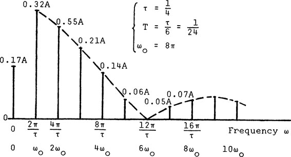
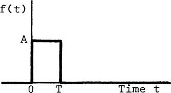
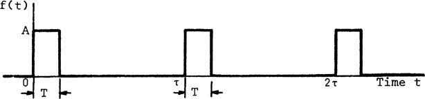
Example C-1. Find the exponential form of the Fourier series for the pulse train shown in Fig. C-l. Plot the frequency spectrum. Assume that the period is $\tau =\raisebox{1ex}{$1$}\!\left/ \!\raisebox{-1ex}{$4$}\right.$ and the pulse duration is T = τ/6.

Solution: The periodic pulse train f(t) is

$\begin{array}{lll}f\left(t\right)=\{\begin{array}{l}0\\ A\\ 0\end{array}\hfill & \text{for}\hfill & \{\begin{array}{l}-\text{τ}/2<t<0\\ 0<t<T\\ T<t<\text{τ}/2\end{array}\hfill \end{array}$

(C-9)

A coefficient c_n of the frequency spectrum is obtained by substituting Eq. C-9 into Eq. C-8.

FIGURE C-1 Rectangular pulse train.

$\begin{array}{llll}{c}_n\hfill & =\frac{1}{\tau }{\displaystyle \underset{-\tau /2}{\int }f\left(t\right)e^{-jn{\text{ω}}_{0}t}dt}\hfill & =\frac{1}{\tau }{\displaystyle \underset{0}{\overset{T}{\int }}A{e}^{-jn\left(2n/\tau \right)t}dt}\hfill & \tau /2\hfill \\ \hfill & =\hfill & \frac{A}{n\pi }\left(\sin \frac{n\pi T}{\tau }\right)e^{-jn\pi T/\tau }\hfill & \hfill \end{array}$

(C-10)

$\begin{array}{lll}\left|c_n\right|=\frac{A}{n\pi }\left|\sin \frac{n\pi T}{\tau }\right|\hfill & \text{or}\hfill & \left|c_n\right|=\frac{AT}{\tau }\left|\sin \frac{\left(n\pi T/\tau \right)}{n\pi T/\tau }\right|\hfill \end{array}$

(C-11)

The exponential form of the Fourier series is formed by substituting Eq. C-10 into Eq. C-7.

$f\left(t\right)=\frac{A}{\pi }{\displaystyle \sum _{n=-\infty }^{\infty }\frac{1}{n}\left(\sin \frac{n\pi T}{\tau }\right)e^{jn\left(2\pi /\tau \right)\left(t-T/2\right)}}$

(C-12)

where ω₀ = 2π/τ. Note that the magnitude d_n for the frequency spectrum from Eq. 4-78 (Chapter 4) is two times that of |c_n| from Eq. C-5, and d_n is used for the plot in Fig. C-2. The value of c₀ is deduced from Eq. C-10 by l’Hospital’s rule.

$c_0=\underset{n\to 0}{\lim }\frac{A}{n\pi }\sin \frac{n\pi T}{\tau }=A\frac{T}{\tau }$

C-2. FOURIER INTEGRAL AND TRANSFORM PAIR

A transient is nonrepeating. It can be regarded as a periodic function with an extremely long period. A heuristic derivation of the Fourier integral is given in this section.

FIGURE C-2 Frequency spectrum of rectangular pulse train shown in Fig. C-l.

A periodic function has a discrete spectrum as illustrated in Fig. C-2. The interval between adjacent components in a spectrum is Δω = ω₀, where ω₀ is the fundamental frequency in rad/s. The frequencies of the kth and the (k + l) st components are

$\begin{array}{lll}k{\text{ω}}_0=k\frac{2\pi }{\tau }\underset{\_}{\underset{\_}{\Delta }}{\text{ω}}_k\hfill & \text{and}\hfill & \left(k+1\right){\text{ω}}_0=\left(k+1\right)\frac{2\pi }{\tau }\underset{\_}{\underset{\_}{\Delta }}{\text{ω}}_{k+1}\hfill \end{array}$

(C-13)

$\Delta \text{ω=}\left(k+1\right)\frac{2\pi }{\tau }-k\frac{2\pi }{\tau }=\frac{2\pi }{\tau }$

(C-14)

A typical Fourier coefficient c_k in Eq. C-8 is at the frequency kω₀. Using the notation c(ω_k) for c_k, and ω_k for kω₀, and substituting 1/τ = Δω/2π into Eqs. C-7 and Eq. C-8, we get

$\begin{array}{llll}f\left(t\right)\hfill & =\hfill & {\displaystyle \sum _{k=-\infty }^{\infty }c\left({\text{ω}}_k\right)e^{-j{\omega }_{k}t}}\hfill & \hfill \\ c\left({\text{ω}}_k\right)\hfill & =\hfill & \frac{\Delta \text{ω}}{2\text{π}}{\displaystyle \underset{-\tau /2}{\int }f\left(t\right)e^{-j{\text{ω}}_{k}t}dt}\hfill & \tau /2\hfill \\ f\left(t\right)\hfill & =\hfill & {\displaystyle \sum _{k=-\infty }^{\infty }\left[\frac{\Delta \text{ω}}{2\text{π}}{\displaystyle \underset{-\tau /2}{\int }f\left(t\right)e^{-j{\text{ω}}_{k}t}dt}\right]e^{j{\text{ω}}_{k}t}}\hfill & \tau /2\hfill \end{array}$

(C-15)

As the period τ approaches infinity, Δω becomes dω in Eq. C-14, and the discrete spectrum in Fig. C-2 becomes a continuous spectrum. At the same time, the discrete variable ω_k in Eq. C-15 becomes a continuous variable ω, and the summation becomes an integration. Thus Eq. C-15 becomes the Fourier integral of the transient f(t).

$f\left(t\right)=\frac{1}{2\pi }{\displaystyle \underset{-\infty }{\overset{\infty }{\int }}\left[{\displaystyle \underset{-\infty }{\overset{\infty }{\int }}f\left(t\right)e^{-j\text{ωt}}dt}\right]}{e}^{j\text{ωt}}d\text{ω}$

(C-16)

Defining the quantity inside the brackets as g(jω), we obtain the Fourier transform pair:

$f\left(t\right)=\frac{1}{2\text{π}}{\displaystyle {\int }_{-\infty }^{\infty }g\left(j\text{ω}\right)e^{j\text{ω}t}d\text{ω}}={ℱ}^{-1}\left[g\left(j\text{ω}\right)\right]$

(C-17)

$g\left(j\text{ω}\right)={\displaystyle {\int }_{-\infty }^{\infty }f\left(t\right)e^{-j\text{ω}t}dt}=ℱ\left[f\left(t\right)\right]$

(C-18)

where g(jω) is the Fourier transform $ℱ\left[f\left(t\right)\right]$ and f(t)is the inverse transform ${ℱ}^{-1}\left[g\left(j\text{ω}\right)\right]$.

The transform pair describes a physical event in two equivalent domains, where f(t)is in the time domain and g(jω) in the frequency domain. A problem can be analyzed in either domain and the results are mutually convertable. Hence it is possible to speak of the frequency content of a transient signal in Sec. 4-8.

The Fourier transform g(jω) is a complex function of ω. Expanding e^−jωt in Eq. C-18 as a sine and cosine function gives

$g\left(j\text{ω}\right)={\displaystyle {\int }_{-\infty }^{\infty }f\left(t\right)\cos \text{ω}tdt}-j{\displaystyle {\int }_{-\infty }^{\infty }f\left(t\right)\sin \text{ω}tdt}$

(C-19)

$g\left(j\text{ω}\right)=\mathrm{Re}\left[g\left(j\text{ω}\right)\right]+j\mathrm{Im}\left[g\left(j\text{ω}\right)\right]$

(C-20)

where Re[g(jω)] is the real part and Im[g(jω)] the imaginary part of the Fourier transformation g(jω). Hence

$\left|g\left(j\text{ω}\right)\right|=\left|\mathrm{Re}\left[g\left(j\text{ω}\right)\right]+j\mathrm{Im}\left[g\left(j\text{ω}\right)\right]\right|$

(C-21)

$/g\left(j\text{ω}\right)={\tan }^{-1}\frac{\mathrm{Im}\left[g\left(j\text{ω}\right)\right]}{\mathrm{Re}\left[g\left(j\text{ω}\right)\right]}$

(C-22)

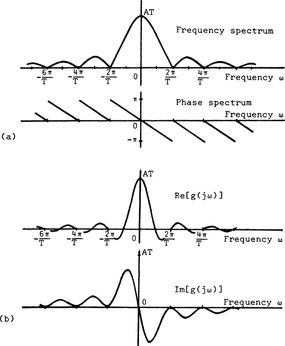
Example C-2. (a) Determine the Fourier transform g(jω) of the non-periodic rectangular pulse f(t) in Fig. C-3, where

$\begin{array}{ll}f\left(t\right)=\{\begin{array}{l}A\\ 0\end{array}\hfill & \text{for}\{\begin{array}{l}0<t<T\\ \text{everywhere else}\end{array}\hfill \end{array}$

(b) Plot the corresponding Re[g(jω)] and Im[g(jω)].

Solution: (a) Substituting f(t) in Eq. C-18, we get

$\begin{array}{lll}g\left(j\text{ω}\right)\hfill & =\hfill & {\displaystyle {\int }_0^{T}A{e}^{-j\text{ω}t}dt}=\frac{A}{j\text{ω}}\left(1-e^{-j\text{ωT}}\right)\hfill \\ \hfill & =\hfill & \frac{A}{j\text{ω}}\left(e^{+j\text{ωT}/2}-e^{-j\text{ω}T/2}\right)e^{-j\text{ω}T/2}\hfill \\ \hfill & =\hfill & \frac{2A}{\text{ω}}\left(\sin \frac{\text{ω}T}{2}\right)e^{-j\text{ω}T/2}\hfill \\ \hfill & =\hfill & AT\frac{\sin \text{ω}T/2}{\text{ω}T/2}{e}^{-j\text{ω}T/2}\hfill \end{array}$

(C-23)

FIGURE C-3 Rectangular pulse.

(b) Substituting e^−jωT/2 = (cos ωT/2 – j sin ωT/2) in Eq. C-23 yields

$\begin{array}{lll}g\left(j\text{ω}\right)\hfill & =\hfill & \frac{2A}{\text{ω}}\left(\sin \frac{\text{ω}T}{2}\right)\left(\cos \frac{\text{ω}T}{2}-j\sin \frac{\text{ω}T}{2}\right)\hfill \\ \hfill & =\hfill & \frac{A}{\text{ω}}\sin \text{ω}T+j\frac{A}{\text{ω}}\left(\cos \text{ω}T-1\right)\hfill \\ \hfill & =\hfill & \left(AT\frac{\sin \text{ω}T}{\text{ω}T}\right)+j\left(AT\frac{\cos \text{ω}T-1}{\omega T}\right)\hfill \\ \hfill & =\hfill & \mathrm{Re}\left[g\left(j\text{ω}\right)\right]+j\mathrm{Im}\left[g\left(j\text{ω}\right)\right]\hfill \end{array}$

(C-24)

The frequency spectrum |g(jω)| versus frequency ω and the phase spectrum/g(jω) versus ω plots are shown in Fig. C-4a. The Re[g(jω)] and Im[g(jω)] parts are shown in Fig. C-4b.

C-3. INVERSE TRANSFORMATION

The transient f(t)is obtained from the inverse Fourier transform of g(jω) shown in Eq. C-17. The simplified inverse transformation and the properties of g(jω) are described in this section.

The integration in Eq. C-17 is simplified by assuming that f(t) is a realtime function, and f(t) = 0 for t < 0. Expanding g(jω) and e^jωt in Eq. C-17 gives

$\begin{array}{lll}f\left(t\right)\hfill & =\hfill & \frac{1}{\text{2π}}{\displaystyle {\int }_{-\infty }^{\infty }\left\{\mathrm{Re}\left[g\left(j\text{ω}\right)\right]+j\mathrm{Im}\left[g\left(j\text{ω}\right)\right]\right\}\left(\text{cos}\text{ω}t+j\sin \text{ω}t\right)}\hfill \\ \hfill & =\hfill & \frac{1}{\text{2π}}{\displaystyle {\int }_{-\infty }^{\infty }\left\{\mathrm{Re}\left[g\left(j\text{ω}\right)\right]\text{cos}\text{ω}t-\mathrm{Im}\left[g\left(j\text{ω}\right)\right]\sin \text{ω}t\right\}d\text{ω}}\hfill \\ \hfill & \hfill & +\frac{j}{\text{2π}}{\displaystyle {\int }_{-\infty }^{\infty }\left\{\mathrm{Re}\left[g\left(j\text{ω}\right)\right]\sin \text{ω}t+\mathrm{Im}\left[g\left(j\text{ω}\right)\right]\text{cos}\text{ω}t\right\}d\text{ω}}\hfill \end{array}$

(C-25)

From the assumption that f(t)is a real-time function, the imaginary part of f(t) in Eq. C-25 is zero. Note that the quantities in Eq. C-25 are functions of ω. The imaginary part has two terms in the integrand, and each must be an odd function of ω for the integral to be zero for −∞ < ω < ∞. Since sin ωt is an odd function, Re[g(jω)] must be an even function of ω. Similarly, cos ωt is an even function and Im[g(jω)] is an odd function of ω.

From the assumption that f(t)= 0 for t < 0, the real part of f(t) in Eq. C-25 must be zero for t < 0. The real part has two terms in the integrand. The {Re[g(jω)] cos ωt} term is an even function of t and {Im[g(jω)] sin ωt} is an odd function of t. Their integrals for t < 0 must be equal and opposite to yield f(t)= 0 for t < 0. Furthermore, if these terms are even and odd functions of t, their integrals must be identical for t > 0. Finally, each term is an even function of ω, and the integration can be carried out over half of the rangefor 0 > ω > ∞.

FIGURE C-4 Fourier transform g(jω)of rectangular pulse shown in Fig. C-3.

By assuming that f(t) is a real-time function and f(t) = 0 for t < 0, the simplified form of Eq. C-17 is

$\begin{array}{cc}f\left(t\right)=\frac{2}{\text{π}}{\displaystyle {\int }_0^{\infty }\mathrm{Re}\left[g\left(j\text{ω}\right)\right]\text{cos}\text{ω}td\text{ω}}& \text{for }t>0\end{array}$

(C-26)

or

$\begin{array}{ccc}f\left(t\right)=-\frac{2}{\text{π}}{\displaystyle {\int }_0^{\infty }\mathrm{Im}\left[g\left(j\text{ω}\right)\right]\sin \text{ω}td\text{ω}}& \text{for }t& 0\end{array}$

(C-27)

Since the real and imaginary parts of g(jω) are even and odd functions of ω, the following properties are self-evident:

$\begin{array}{c}\mathrm{Re}\left[g\left(-j\text{ω}\right)\right]=\mathrm{Re}\left[g\left(j\text{ω}\right)\right]\\ \mathrm{Im}\left[g\left(-j\text{ω}\right)\right]=-\mathrm{Im}\left[g\left(j\text{ω}\right)\right]\\ \left|g\left(-j\text{ω}\right)\right|=\left|g\left(j\text{ω}\right)\right|\\ /g\left(-j\text{ω}\right)=-/g\left(j\text{ω}\right)\\ g\left(-j\text{ω}\right)=g^{\ast }\left(j\text{ω}\right)\end{array}$

(C-28)

where g*(jω) is the complex conjugate of g(jω). The first four properties above for a rectangular pulse are shown in Fig. C-4.

C-4. ILLUSTRATION FOR OBTAINING THE FOURIER TRANSFORM

Fourier transformation and the inverse are routinely performed by digital computes. An analog method for obtaining the transformation is described to give a better feeling for the subject.

The Fourier transform g(jω) of a transient f(t) is computed by means of Eq. C-19. Assuming that f(t) = 0 for t < 0, we get

$g\left(j\text{ω}\right)={\displaystyle {\int }_0^{\infty }f\left(t\right)\text{cos ω}tdt}-j{\displaystyle {\int }_0^{\infty }f\left(t\right)\sin \text{ω}tdt}$

(C-29)

$\mathrm{Re}\left[g\left(j\text{ω}\right)\right]={\displaystyle {\int }_0^{\infty }f\left(t\right)\text{cosω}tdt}$

(C-30)

$-\mathrm{Im}\left[g\left(j\text{ω}\right)\right]={\displaystyle {\int }_0^{\infty }f\left(t\right)\sin \text{ω}tdt}$

(C-31)

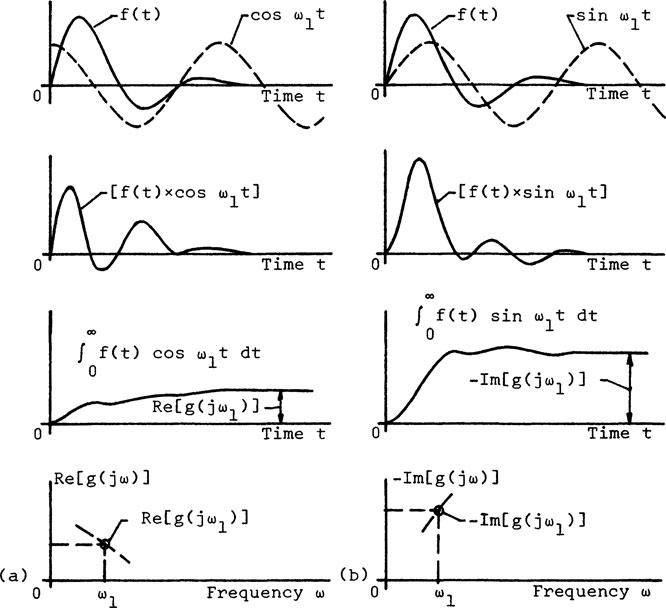
Assume a transient f(t) as shown in Fig. C-5a. Re[g(jω)] from Eq. C-30 is integrated with respect to time t with ω to as a parameter. For a given ω = ω₁, the multiplication and integration are as shown in the figure. A value Re[g(jω₁)] is obtained when the integral reaches a constant value. The process is repeated for a range of ω to obtain Re[g(jω)] versus ω. Only positive values of ω need be considered, since Re[g(jω)] is an even function. Similarly, Im[g(jω)] can be computed as shown in Fig. C-5b.

The same procedure is used for finding the inverse transform for a given g(jω), using the time t as a parameter. Either Eq. C-26 or Eq. C-27 can be used for the computation.

FIGURE C-5

Suggested Readings

Hsu, W. P., Fourier Analysis, Simon and Schuster, New York, 1967.

Papoulis, A., The Fourier Integral and Its Applications, McGraw-Hill Book Company, New York, 1962.

Sneddon, L. N., Fourier Transforms, McGraw-Hill Book Company, New York, 1951.

Stuart, R. D., An Introduction to Fourier Analysis, John Wiley & Sons, Inc., New York, 1966.