Getting Started with the Survey Documentation and Analysis Software
Survey Documentation and Analysis (SDA) is open-source software that is used for online dissemination of data from many surveys and censuses, including the U.S. Decennial Census, the American Community Survey, and the Current Population Survey, all of which are collected by the U.S. Census Bureau and distributed through the Integrated Public Use Microdata Series (IPUMS). SDA is also used to disseminate data from large ongoing research projects such as the General Social Survey and the American National Election Study (see chapter 23). SDA allows users to do many types of statistical analyses (regressions, correlations, etc.) on data sets without downloading the data or using a desktop statistical program such as SPSS or Stata. For reference librarians, its most useful feature is its ability to make custom tables, called “crosstabulations” in statistics jargon.
Only website administrators can load data sets into SDA, so you can analyze a data set with SDA only if an organization such as IPUMS or the Interuniversity Consortium for Political and Social Research (ICPSR) has that data set up for SDA access. Look on these organizations’ websites for links that say something such as “Analyze data online” or “Analyze data using SDA.” On many of these sites, you are asked to create a free account, log in, and agree to certain terms of use before accessing the data via SDA.
By default, SDA should open in the “Frequencies/Crosstabulations Program,” which allows you to create tables. If you are an advanced user and want to do other types of analyses, such as correlations or regressions, you can access those options under the “Analysis” menu in the upper left. This guide does not cover those analyses.
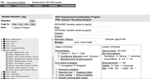
In SDA, the variables are listed in the left column, and the table-building options are in the right column (see figure 1). The first step is to find the variables you need in the left column. If you want more information about any given variable, click on it; this copies the variable name into the “Selected” box at the top of the left column. Then click the “View” button next to the “Selected” box to see details about the variable. These details may include the full text of the question asked and always include the possible responses and the numeric codes used for each response (see figure 2).
To use a particular variable in constructing your table, close the “View” window and click one of the “Copy to” buttons underneath the “Selected” box. There are four “Copy to” buttons, one for each of the options for using a variable in constructing a table. “Row” and “Column” simply place that variable in either the rows or the columns of the table. “Control” creates separate tables for each of the possible values for that variable. For example, using “sex” as the control variable creates separate tables with the responses for men and women (assuming that the survey had a variable named “sex” with that information). “Filter” allows you to limit which groups are included in the table. For example, instead of using “sex” as a control variable, you could use it as a filter variable and view only the responses of women.

FIGURE 1
The final variable-related option in SDA is “Weight.” Many surveys use weight variables to compensate for the fact that their surveys are not simple random samples. If you have ever taken an introductory statistics course, you probably remember your professor emphasizing that the tests you learned were appropriate only for samples randomly chosen from the population, where every person in the population had an equal chance of being selected to be in the study. Few large data sets in the social sciences satisfy this requirement. Thus, since some people have a higher or lower likelihood of participating in the survey, it is appropriate to give their answers more or less weight when calculating statistics that are intended to represent the entire population. Weight variables are used to accomplish this. Often, the survey is set up in SDA to use a weight variable already, in which case you do not need to change anything. Nevertheless, it is always a good idea to look at the weight variable options and make sure that the selected one makes sense. This is especially important when working with multilevel data such as the U.S. Census data, which uses different weight variables for individual-level data (e.g., age, educational attainment) and household-level data (e.g., household income).
There are several “Table Options” and “Chart Options” for changing the format of and adding additional information to the output from SDA. Much of this additional information is intended for more statistically sophisticated users and can safely be ignored when answering the typical “Can you help me find a table with this information?” type of data reference question. Many of the other options are self-explanatory, such as including the question text or changing the type of chart created. If you are curious about any of these options, just click on its name to get more information.

FIGURE 2
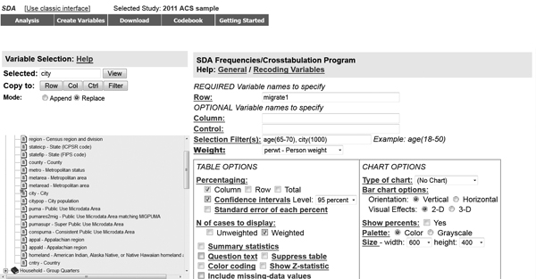
The exception is “Confidence interval.” In my opinion, it is always a good idea to add the confidence interval to your table. The statistics calculated by SDA are estimates, and they come with a margin of error. If you are working with a small sample (which can easily happen if you use the “filter” option to examine a small subset of the population—say, only people living in Delaware, or only people over age 50 with advanced degrees), the margin of error can be quite large. Selecting “confidence interval” as an option adds (depending on your selection) the 90%, 95%, or 99% confidence interval to each cell in the table. This confidence interval, which is presented as a range, gives you information about the precision of each estimate.
For example, I used data from the 2011 American Community Survey, as disseminated through IPUMS, to examine the phenomenon of retirees moving to Florida’s gulf coast. When I looked only at people age 65–70 who lived in the city of Cape Coral (which has a city code of “1000” in this data set), SDA produced an estimate that 91.4 percent of those senior citizens are living in the same house they lived in one year ago; 5.0 percent had moved from another house in Florida in the past year; 2.8 percent had moved from a house in a different state in the United States, and 0.7 percent had moved from a foreign country (see figures 3 and 4). However, the 95% confidence intervals for those estimates are wide. For example, although the estimate is that 2.8 percent of the 65–70-year-olds living in Cape Coral had moved there from another state in the previous year, the 95% confidence interval is 1.0–8.1 percent. That means that there is a 95 percent chance that the true figure—the percentage you would find if you asked this question of every single 65–70-year-old living in Cape Coral—is somewhere between 1.0 and 8.1 percent, and a 5 percent chance that the true figure is less than 1.0 percent or greater than 8.1 percent.

FIGURE 3
Compare this to the 95% confidence interval if one generates the same table for people age 65–70 living in the entire state of Florida. In this case, the estimate is 2.6 percent, but the 95% confidence interval is 2.4–2.9 percent (see figure 5). Even the 99% confidence interval is only 2.3–3.0 percent. For the entire state of Florida, we can say with near-complete confidence that the percentage of the population age 65–70 who moved from another U.S. state to Florida last year is between 2.3 and 3.0 percent. For the city of Cape Coral, we can be much less confident about the true percentage.

FIGURE 4
When you have selected all the options you want, click the “Run the Table” button to create your data table.

FIGURE 5