In constructive mathematics, a problem is counted as solved only if an explicit solution can, in principle at least, be produced. Thus, for example, “There is an x such that P(x)” means that, in principle at least, we can explicitly produce an x such that P(x). If the solution to the problem involves parameters, we must be able to present the solution explicitly by means of some algorithm or rule when given values of the parameters. That is, “for every x there is a y such that P(x, y) means that, we possess an explicit method of determining, for any given x, a y for which P(x, y). This leads us to examine what it means for a mathematical object to be explicitly given.
9.1 The Constructive Real Number Line1
To begin with, everybody knows what it means to give an integer explicitly. For example, 7 ⋅ 104 is given explicitly, while the number n defined to be 0 if an odd perfect number exists, and 1 if an odd perfect number does not exist, is not given explicitly. The number of primes less than, say, 101000000 is given explicitly, in the sense intended here, since we could, in principle at least, calculate this number. Constructive mathematics as we shall understand it is not concerned with questions of feasibility, nor in particular with what can actually be computed in real time by actual computers. Rational numbers may be defined as pairs of integers (a, b) without a common divisor (where b > 0 and a may be positive or negative, or a is 0 and b is 1). The usual arithmetic operations on the rationals, together with the operation of taking the absolute value, are then easily supplied with explicit definitions. Accordingly it is clear what it means to give a rational number explicitly. To specify exactly what is meant by giving a real number explicitly is not quite so simple. For a real number is by its nature an infinite object, but one normally regards only finite objects as capable of being given explicitly. This difficulty may be overcome by stipulating that, to be given a real number, we must be given a (finite) rule or explicit procedure for calculating it to any desired degree of accuracy. Intuitively speaking, to be given a real number r is to be given a method of computing, for each positive integer n, a rational number r n such that


 for all p. Clearly r # s implies r ≠ s, but the converse cannot be affirmed constructively.3
Is it constructively the case that for any real numbers x and y, we have x = y ∨ x ≠ y? The answer is no. For if this assertion were constructively true, then, in particular, we would have a method of deciding whether, for any given rational number r, whether r = π√2 or not. But at present no such method is known—it is not known, in fact, whether π√2 is rational or irrational. We can, of course, calculate π√2 to as many decimal places as we please, and if in actuality it is unequal to a given rational number r, we shall discover this fact after a sufficient amount of calculation. If, however, π√2 is equal to r, even several centuries of computation cannot make this fact certain; we can be sure only that its value is very close to r. We have no method which will tell us, in finite time, whether π√2 exactly coincides with r or not. This situation may be summarized by saying that equality on the reals is not decidable . (By contrast, equality on the integers or rational numbers is decidable.) Observe that this does not mean ¬(x = y ∨ x ≠ y). We have not actually derived a contradiction from the assumption x = y ∨ x ≠ y; we have only given an example showing its implausibility. It is natural to ask whether it can actually be refuted. For this it would be necessary to make some assumption concerning the real numbers which contradicts classical mathematics. Certain schools of constructive mathematics are willing to make such assumptions; but the majority of constructivists confine themselves to methods which are also classically correct.4
Despite the fact that constructive equality of real numbers is not a decidable
relation, it is
stable
5 in the sense of satisfying the law
of double negation
¬(r ≠ s) ⇒ r = s. In fact, we can prove the stronger assertion that ¬(r # s) ⇒ r = s. For, given k, we may choose n so that  and
and  for all p. If
  , then we would have
  for all p, which entails r ≠ s. If ¬(r # s), it follows that
  and
and  for every p. Since for every k we can find n so that this inequality holds for every p, it follows that r = s.
6
for every p. Since for every k we can find n so that this inequality holds for every p, it follows that r = s.
6
One should not, however, conclude from the stability of equality that the law of double negation ¬¬A → A is generally affirmable. That it is not can be seen from the following example. Write the decimal expansion of π and below the decimal expansion ρ = 0.333…, terminating it as soon as a sequence of digits 0123456789 has appeared in π. Then if the 9 of the first sequence 0123456789 in π is the k
th digit after the decimal point,  . Now suppose that ρ were not rational; then
  would be impossible and no sequence 0123456789 could appear in π, so that
  , which is also impossible. Thus the assumption that ρ is not rational leads to a contradiction; yet we are not warranted to assert that ρ is rational, for this would mean that we could calculate integers m and n for which
  . But this evidently requires that we can produce a sequence 0123456789 in π or demonstrate that no such sequence can appear, and at present we can do neither.
9.2 Constructive Meaning of the Logical Operators
p ∧ q: we have a proof of p and a proof of q.
p ∨ q: we have either a proof of p or a proof of q.
¬p: we can derive a contradiction (such as 0 = 1) from p.
p → q: we can convert any proof of p into a proof of q.
∃xp(x): we have a procedure for producing both an object a and a proof that P(a) holds
∀x∈A P(x): we have a procedure which, applied to an object a and a proof that a ∈ A, demonstrates that P(a) holds.
If the symbol “∃” is taken to mean “explicit existence” in the sense indicated above, it cannot be expected to obey the laws of classical logic. For example, ¬∀ is classically equivalent to ∃¬, but the mere knowledge that something cannot always occur does not enable us actually to determine a location where it fails to occur. This is generally the case with existence proofs by contradiction. For instance, consider the following standard proof of the Fundamental Theorem of Algebra: every polynomial p of degree >0 has a (complex) zero. If p lacks a zero, then  is entire and bounded, and so by Liouville’s theorem must be constant. This proof gives no hint of how actually to construct a zero.7
On the basis of these interpretations , in 1930 A. Heyting formulated the axioms of intuitionistic (or constructive) logic. 8 This may be presented as a formal system with the following axioms and rules of inference:
Axioms

![$$ \Big[p\to \left(q\to r\right)\to \left[\left(p\to q\right)\to \left(p\to r\right)\right] $$](../images/474107_1_En_9_Chapter/474107_1_En_9_Chapter_TeX_Equg.png)


![$$ \left(p\to r\right)\to \left[\left(q\to r\right)\to \left(p\vee q\to r\right)\right] $$](../images/474107_1_En_9_Chapter/474107_1_En_9_Chapter_TeX_Equk.png)
![$$ \left(p\to q\right)\to \left[\left(p\to \neg q\right)\to \neg p\right] $$](../images/474107_1_En_9_Chapter/474107_1_En_9_Chapter_TeX_Equl.png)


x = x p(x) ∧ x = y → p(y)
Rules of Inference


Classical logic is obtained from intuitionistic logic either by adding as an axiom the law of excluded middle p ∨ ¬p, or the law of double negation ¬¬p → p. The chief difference between classical and intuitionistic logic is that in the latter neither of these two laws are generally affirmed.
9.3 Order on the Constructive Reals

We observe that r # s ⇔ r < s ∨ s < r. The implication from right to left is clear. Conversely, suppose that r # s. Find n and k so that  for every p, and determine m > n so that
  and
and  for every p. Either
  or
or  ; in the first case
  for every p, whence s < r; similarly, in the second case, we obtain r < s.
We define r ≤ s to mean that s < r is false. Notice that r ≤ s is not the same as r < s or r = s: in the case of the real number
ρ defined above, for instance, clearly  ; but we do not know whether
  or
or  . Still, it is true that r ≤ s ∧ s ≤ r ⇒ r = s. For the premise is the negation of r < s ∨ s < r, which, by the above, is equivalent to ¬r # s. But we have already seen that this last implies r = s.
There are several common properties of the order relation on real numbers which hold classically but which cannot be established constructively. Consider, for example, the trichotomy law x < y ∨ x = y ∨ y < x. Suppose we had a method enabling us to decide which of the three alternatives holds. Applying it to the case y = 0, x = π√2 – r for rational r would yield an algorithm for determining whether π√2 = r or not, which we have already observed is an open problem. One can also demonstrate the failure of the trichotomy law (as well as other classical laws) by the use of “fugitive sequences ”. Here one picks an unsolved problem of the form ∀nP(n), where P is a decidable property of integers—for example, Goldbach’s conjecture that every even number ≥ 4 is the sum of two odd primes. Now one defines a sequence—a “fugitive” sequence—of integers (n k) by n k = 0 if 2 k is the sum of two primes and n k = 1 otherwise. Let r be the real number defined by r k = 0 if n k = 0 for all j ≤ k, and r k = 1/m otherwise, where m is the least positive integer such that n m = 1. It is then easy to check that r ≥ 0 and r = 0 if and only if Goldbach’s conjecture holds. Accordingly the correctness of the trichotomy law would imply that we could resolve Goldbach’s conjecture. Of course, Goldbach’s conjecture might be resolved in the future, in which case we would merely choose another unsolved problem of a similar form to define our fugitive sequence .
A similar argument shows that the law r ≤ s ∨ s ≤ r also fails constructively: define the real number s by s k = 0 if n k = 0 for all j ≤ k; s k = 1/m if m is the least positive integer such that n m = 1, and m is even; s k = −1/m if m is the least positive integer such that n m = 1, and m is odd. Then s ≤ 0 (resp. 0 ≤ s) would mean that there is no number of the form 2 ⋅ 2k (resp. 2 ⋅ (2k + 1)) which is not the sum of two primes. Since neither claim is at present known to be correct, we cannot assert the disjunction s ≤ 0 ∨ 0 ≤ s.

9.4 Algebraic Operations on the Constructive Reals
r + s is the sequence (r n + s n)
r – s is the sequence (r n – s n)
r ⋅ s or rs is the sequence (r n s n)
if r # 0, r −1 is the sequence (t n), where t n = r n −1 if t n ≠ 0 and t n = 0 if r n = 0
|r| is the sequence (|r n|)
 and
and  for every p, so that
  for every p, and rs # 0. Conversely, if rs # 0, then we can find k and n so that

But it is not constructively true that, if rs = 0, then r = 0 or s = 0! To see this, use the following prescription to define two real numbers
r and s. If in the first n decimals of π no sequence 0123456789 occurs, put r
n = s
n = 2–n; if a sequence of this kind does occur in the first n decimals, suppose the 9 in the first such sequence is the k
th digit. If k is odd, put r
n = 2–k, s
n = 2–n; if k is even, put r
n = 2–n, s
n = 2–k. Then we are unable to decide whether r = 0 or s = 0. But rs = 0. For in the first case above r
n s
n = 2–2n; in the second r
n s
n = 2–k–n. In either case  , so that rs = 0.
9.5 Convergence of Sequences and Completeness of the Constructive Reals
As usual, a sequence (a n) of real numbers is said to converge to a real number b, or to have limit s if, given any natural number k, a natural number n can be found so that for every natural number p,

As in classical analysis, a constructive necessary and condition that a sequence (a n) of real numbers be convergent is that it be a Cauchy sequence, that is, if, given any given any natural number k, a natural number n can be found so that for every natural number p,

But some classical theorems concerning convergent sequences are no longer valid constructively. For example, a bounded momotone sequence need no longer be convergent. A simple counterexample is provided by the sequence (a n) defined as follows: a n = 1–2–n if among the first n digits in the decimal expansion of π no sequence 0123456789 occurs, while a n = 2–2–n if among these n digits such a sequence does occur. Since it is not known whether the limit of this sequence, if it exists, is 1 or 2, we cannot claim that that this limit exists as a well defined real number .
In classical analysis ℝ is complete in the sense that every nonempty set of real numbers that is bounded above has a supremum . As it stands, this assertion is constructively incorrect. For consider the set A of members {x 1, x 2, …} of any fugitive sequence of 0 s and 1 s. Clearly A is bounded above, and its supremum would be either 0 or 1. If we knew which, we would also know whether x n = 0 for all n, and the sequence would no longer be fugitive.
However, the completeness of ℝ can be salvaged by defining suprema and infima somewhat more delicately than is customary in classical mathematics. A nonempty set A of real numbers is bounded above if there exists a real number b, called an upper bound for A, such that x ≤ b for all x ∈ A. A real number b is called a supremum, or least upper bound, of A if it is an upper bound for A and if for each ε > 0 there exists x ∈ A with x > b – ε. We say that A is bounded below if there exists a real number b, called a lower bound for A, such that b ≤ x for all x ∈ A. A real number b is called an infimum, or greatest lower bound, of A if it is a lower bound for A and if for each ε > 0 there exists x ∈ A with x < b + ε. The supremum (respectively, infimum) of A, is unique if it exists and is written sup A (respectively, inf A).
Let us prove the constructive least upper bound principle .
Theorem
Let A be a nonempty set of real numbers that is bounded above. Then sup A exists if and only if for all x, y ∈ ℝ with x < y, either y is an upper bound for A or there exists a ∈ A with x < a.
Proof
If sup A exists and x < y, then either sup A < y or x < sup A; in the latter case we can find a ∈ A with sup A – (sup A – x) < a, and hence x < a. Thus the stated condition is necessary.


An analogous result for infima can be stated and proved in a similar way.
9.6 Functions on the Constructive Reals
Considered constructively , a function from ℝ to ℝ is a rule F which enables us, when given a real number x, to compute another real number F(x) in such a way that, if x = y, then F(x) = F(y). It is easy to check that every polynomial is a function in this sense, and that various power series and integrals , for example those defining tan x and e x, also determine functions.
Viewed constructively, some classically defined “functions” on ℝ can no longer be considered to be defined on the whole of ℝ. Consider, for example, the “blip” function B defined by B(x) = 0 if x ≠ 0 and B(0) = 0. Here the domain of the function is {x∈ ℝ: x = 0 ∨ x ≠ 0}. But we have seen that we cannot assert dom(B) = ℝ. Accordingly, the blip function is not well defined as a function from ℝ to ℝ. Of course, classically, B is the simplest discontinuous function defined on ℝ. The fact that the simplest possible discontinuous function fails to be defined on the whole of ℝ gives grounds for the suspicion that no function defined on ℝ can be discontinuous; in other words, that, constructively speaking, all functions defined on ℝ are continuous. 9 The claim is plausible. For if a function F is well-defined on all reals x, it must be possible to compute the value for all rules x determining real numbers , that is, determining their sequences of rational approximations x 1, x 2, … . Now F(x) must be computed to accuracy ε in a finite number of steps—the number of steps depending on ε. This means that only finitely many approximations can be used, i.e., F(x) can be computed to within ε only when x is known within δ for some δ. Thus F should indeed be continuous. In fact all known examples of constructive functions defined on ℝ are continuous.
Constructively, a real-valued function f is continuous if for each ε > 0 we can find a specific δ > 0 such that |f(x) – f(y)| ≤ ε whenever |x – y| < δ. If all functions on ℝ are continuous, then a subset A of ℝ may fail to be genuinely complemented: that is, there may be no subset B of ℝ disjoint from A such that ℝ = A ∪ B.
To see this, we first suppose that A, B are disjoint subsets of ℝ and that there is a point a ∈ A which can be approached arbitrarily closely by points of B (or vice-versa). Then, assuming all functions on ℝ are continuous, it cannot be the case that ℝ = A ∪ B. For if so, we may define the function f on ℝ by f(x) = 0 if x ∈ A, f(x) = 1 if x ∈ B. Then for all δ > 0 there is b ∈ B for which |b – a| < δ, but |f(b) – f(a)| = 1. Thus f fails to be continuous at a, and we conclude that ℝ ≠ A ∪ B.
Now if we take A to be any fini te set of real numbers, any union of open or closed intervals, or the set ℚ of rational numbers, then in each case the set B of points “outside” A satisfies the above condition. Accordingly, for each such subset A, ℝ is not “decomposable” into A and the set of points “outside” A, in the sense that these two sets of points together do not exhaust ℝ. This fact indicates that the constructive continuum is a great deal more “cohesive ” than its classical counterpart. For classically, the continuum is merely connected in the sense that it is not (nontrivially) decomposable into two open (or closed) subsets. Constructively, however, ℝ is indecomposable into subsets which are neither open nor closed. Indeed, in some formulations of constructive analysis ,10 ℝ (and all of its intervals) is cohesive in the stronger sense that it cannot be decomposed in any way whatsoever. 11 In this sense the constructive real line can be brought close to the ideal of a true continuum.
 and the other at
  and of approximately the same value. Now arrange things so that
  and
and  , where t is some small parameter. If we could tell where f assumes its absolute maximum, clearly we could also determine whether t ≤ 0 or t ≥ 0, which, as we have seen, is not, in general, possible. Nevertheless, it can be shown that from f we can in fact calculate the maximum value itself, so that at least one can assert the existence of that maximum, even if one can’t tell exactly where it is assumed.
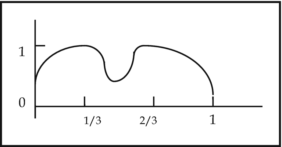
Caption
 and
and  . If the intermediate value theorem held, we could determine a for which f(a) = 0. Then either
  or
or  ; in the former case t ≥ 0; in the latter t ≤ 0. Thus we would be able to decide whether t ≥ 0 or t ≤ 0; but we have seen that this is not constructively possible in general.
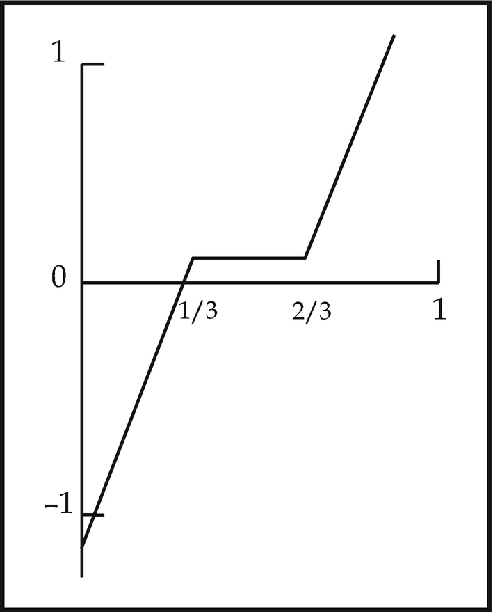
Caption

![$$ \forall f\left[P(f)\to \exists x\left(f(x)=0\right)\right]. $$](../images/474107_1_En_9_Chapter/474107_1_En_9_Chapter_TeX_Equab.png)
9.7 Axiomatizing the Constructive Reals
a binary relation > (greater than)
a corresponding apartness relation # defined by x # y ⇔ x > y or y > x
a unary operation x ↦ −x
binary operations (x, y) ↦ x + y (addition) and (x, y) ↦ xy (multiplication)
distinguished elements 0 (zero) and 1 (one) with 0 ≠ 1
a unary operation x ↦ x −1 on the set of elements ≠ 0.

The sets N of natural numbers, N + of positive integers, Z of integers and Q of rational numbers are identified with the usual subsets of R; for instance N + is identified with the set of elements of R of the form 1 + 1 + ⋯ + 1.
These relations and operations are subject to the following three groups of axioms, which, taken together, form the system CA of axioms for constructive analysis , or the constructive real numbers.
Field Axioms


Order Axioms


Notice that from the fourth of the order axioms it follows that ¬(x ≠ y) → x = y, 13 that is, the equality relation is stable .
b is an upper bound for S, and
for each c < b there exists s ∈ S with s > c.
Special Properties of >
Archimedean axiom. For each x ∈ R such that x ≥ 0 there exists n ∈ N such that
x < n.
The least upper bound principle. Let S be a nonempty subset of R that is bounded above, such that for all real numbers a, b with a < b, either b is an upper bound for S or else there exists s ∈ S with s > a. Then S has a least upper bound.


The constructive real line ℝ as introduced above is a model of CA . Are there any other models, that is, models not isomorphic to ℝ? If classical logic is assumed, CA is a categorical theory and so the answer is no. But this is not the case within intuitionistic logic , for it can be shown that, in a topos, both the Dedekind and Cantor reals are models of CA, while, as has been pointed out above, these may fail to be isomorphic.
9.8 The Intuitionistic Continuum
In constructive analysis , a real number is an infinite (convergent) sequence of rational numbers generated by an effective rule, so that the constructive real line is essentially just a restriction of its classical counterpart. Brouwerian intuitionism takes a more imaginative view of the matter, resulting in a considerable enrichment of the arithmetical continuum over the version offered by strict constructivism. As conceived by intutionism, the arithmetical continuum admits as real numbers “not only infinite sequences determined in advance by an effective rule for computing their terms, but also ones in whose generation free selection plays a part .”16 The latter are called (free) choice sequences . Without loss of generality we may and shall assume that the entries in choice sequences are natural numbers.
In Brouwer’s analysis, the individual place in the continuum, the real number, is to be defined not by a set but by a sequence of natural numbers, namely, by a law which correlates with every natural number n a natural number φ(n)… How then do assertions arise which concern… all real numbers , i.e., all values of a real variable? Brouwer shows that frequently statements of this form in traditional analysis, when correctly interpreted, simply concern the totality of natural numbers. In cases where they do not, the notion of sequence changes its meaning: it no longer signifies a sequence determined by some law or other, but rather one that is created step by step by free acts of choice, and thus necessarily remains in statu nascendi. This “becoming” selective sequence (werdende Wahlfolge) represents the continuum, or the variable, while the sequence determined ad infinitum by a law represents the individual real number in the continuum. The continuum no longer appears, to use Leibniz’s language, as an aggregate of fixed elements but as a medium of free “becoming”. Of a selective sequence in statu nascendi, naturally only those properties can be meaningfully asserted which already admit of a yes-or-no decision (as to whether or not the property applies to the sequence) when the sequence has been carried to a certain point; while the continuation of the sequence beyond this point, no matter how it turns out, is incapable of overthrowing that decision. 17
While constructive analysis does not formally contradict classical analysis and may in fact be regarded as a subtheory of the latter, a number of intuitionistically plausible principles have been proposed for the theory of choice sequences which render intuitionistic analysis divergent from its classical counterpart.18 One such principle is Brouwer ’s Continuity Principle. This assderts that, given a relation R (α, n) between choice sequences α and numbers n, if for each α a number n may be determined for which R(α, n) holds, then n can already be determined on the basis of the knowledge of a finite number of terms of α.19 From this one can prove a weak version of the Continuity Theorem, namely, that every function from ℝ to ℝ is continuous.20 Another such principle is Bar Induction , a certain form of induction for well-founded sets of finite sequences.21 Brouwer used Bar Induction and the Continuity Principle in proving his Continuity Theorem that every real-valued function defined on a closed interval is uniformly continuous, from which it follows that the intuitionistic continuum, and all of its closed intervals, are cohesive.22
Brouwer gave the intuitionistic conception of mathematics an explicitly subjective twist by introducing the creative subject . The creative subject was conceived as a kind of idealized mathematician for whom time is divided into discrete sequential stages, during each of which he may test various propositions, attempt to construct proofs, and so on. In particular, it can always be determined whether or not at stage n the creative subject has a proof of a particular mathematical proposition p. While the theory of the creative subject remains controversial, its purely mathematical consequences can be obtained by a simple postulate which is entirely free of subjective and temporal elements.
Now if the construction of these sequences is the only use made of the creative subject , then references to the latter may be avoided by postulating the principle known as Kripke’s Scheme :
a n = 1 if the creative subject has a proof of p at stage n;
a n = 0 otherwise.
For each proposition p there exists an increasing binary sequence <a n> such that p holds if and only if a n = 1 for some n.
Taken together, these principles have been shown23 to have remarkable consequences for the cohesiveness24 of subsets of the continuum. Not only is the intuitionistic continumm cohesive , but, assuming Brouwer ’s Continuity Principle and Kripke’s Scheme, it remains cohesive even if one pricks it with a pin.25 “The [intuitionistic] continuum has, as it were, a syrupy nature, one cannot simply take away one point.”26 If in addition Bar Induction is assumed, then, even more surprisingly, cohesiveness is maintained even when all the rational points are removed from the continuum.
9.9 An Intuitionistic Theory of Infinitesimals
In 1980 Richard Vesley showed that a natural notion of infinitesimal can be developed within intuitionistic mathematics.27 His idea was that an infinitesimal should be a “very small” real number in the sense of not being known to be distinguishable —that is, strictly greater than or less than—zero.
Let α be a variable ranging over choice sequences , x, y variables ranging over real numbers in the intuitionistic continuum R and n a variable ranging over natural numbers. Vesley observes that from Kripke’s scheme one can prove
![$$ \forall \upalpha \exists x\left[\left(x>0\iff \forall n\ \upalpha (n)=0\right)\wedge \left(x>0\iff \neg \forall n\ \upalpha (n)=0\right)\right], $$](../images/474107_1_En_9_Chapter/474107_1_En_9_Chapter_TeX_Equaq.png)
![$$ \forall \upalpha \exists x\left[\right(x\#0\iff \left(\forall n\ \upalpha (n)=0\vee \neg \forall n\ \upalpha (n)=0\right)\Big]. $$](../images/474107_1_En_9_Chapter/474107_1_En_9_Chapter_TeX_Equar.png)
![$$ x\in L\left(\upalpha \right)\iff \left[\right(x\#0\iff \left(\forall n\ \upalpha (n)=0\vee \neg \forall n\ \upalpha (n)=0\right)\Big] $$](../images/474107_1_En_9_Chapter/474107_1_En_9_Chapter_TeX_Equas.png)

The members of L(α) may be considered very small in the sense that they cannot be distinguished from zero unless a decision is made as to whether α is identically zero or not, something which in general cannot be guaranteed. The members of M(α), the α-infinitesimals, are those real numbers which are bounded in absolute value by members of L(α). Notice that the property of being an α-infinitesimal is quite unstable, since in the event of such a decision being made as to whether α is identically zero or not, L(α) automatically becomes identical with the set of reals which can be distinguished from zero and so M(α) with the set of all reals.

The derivative of a function can then be defined in the following way: given f: ℝ → ℝ, the derivative of f at x ∈ℝ is a ∈ ℝ if there is a function g: ℝ → ℝ carrying α-infinitesimals to α-infinitesimals for every α and which also satisfies
