Smooth Infinitesimal Analysis/Synthetic Differential Geometry

10.1 Smooth Worlds

Mathematicians have developed two methods of deriving the theorems of geometry: the analytic and the synthetic. While the analytical method is based on the introduction of numerical coordinates , and so on the theory of real numbers , the (much older) idea behind the synthetic approach is to furnish the subject of geometry with an autonomous foundation within which the theorems become deducible by logical means from an initial body of postulates.

The most familiar examples of the synthetic geometry are classical Euclidean geometry and the synthetic projective geometry introduced by Desargues in the seventeenth century and revived and developed by Poncelet , Steiner and others in the nineteenth century.

The power of analytic geometry derives very largely from the fact that it permits the methods of the calculus, and, more generally, of mathematical analysis, to be introduced into geometry, leading in particular to differential geometry. That being the case, the notion of a “synthetic” differential geometry appears elusive: how can differential geometry be placed on a “purely geometric” or “axiomatic” foundation when the apparatus of the calculus seems to be inextricably involved?

There have been (at least) two attempts to develop a synthetic differential geometry. The first was initiated by Herbert Busemann¹ in the 1940s, building on earlier work of Paul Finsler. Here the idea was to build a differential geometry that, in its author’s words, “requires no derivatives”: the basic objects in Busemann’s approach are not differentiable manifolds, but metric spaces of a certain type in which the notion of a geodesic can be defined in an intrinsic manner.

The second approach, the focus of our attention here, was first proposed in the 1960s by F. W. Lawvere , in his pursuit of a decisive axiomatic framework for continuum mechanics. His ideas have led to the development of a theory now claiming, with good reason, exclusive title to the appellation synthetic differential geometry (SDG).

Since differential geometry “lives” in the category Man of manifolds, it might be supposed that in formulating a “synthetic differential geometry” the category-theorist’s goal would be to find an axiomatic description of Man itself. But in fact the category Man has a couple of “deficiencies” which make it unsuitable as an object of axiomatic description:

1.
It lacks exponentials: that is, the “space of all smooth maps ” from one manifold to another in general fails to be a manifold. And even if it did—
2.
It also lacks “infinitesimal objects”; in particular, there is no “infinitesimal” manifold² Δ for which the tangent bundle Tan M of an arbitrary manifold M can be identified as the exponential “manifold” M ^Δ of all “infinitesimal paths” in M. ³

Lawvere’s idea was to enlarge Man to a category Space —a smooth category or a smooth world, with objects called smooth spaces —through whose introduction these two deficiencies are surmounted, which admits a simple axiomatic description, and is at the same time sufficiently similar to Set to allow mathematical construction and calculation to proceed in the familiar way. Smooth categories are the natural models of SDG.

The essential features of Space are these:

In enlarging Man to Space—in contradistinction to Set—no “new” maps between manifolds are introduced, that is, all maps in Space between objects of Man are smooth⁴ differentiable arbitrarily many times, It is for this reason that analysis in Space is called smooth infinitesimal analysis (SIA) .
Nevertheless, Space, like Set , is a topos. ⁵
But unlike Set, Space has infinitesimal objects. Let R be the smooth real line , that is, the real line considered as an object of Man , and hence also of Space. Then there is a nondegenerate infinitesimal segment Δ of R around 0 which is rigid, that is, remains straight and unbroken under any map in Space . In other words, Δ is subject in Space to Euclidean motions only. If we identify maps on R as curves, then the images of Δ can be considered as “infinitesimal straight segments” of curves.

SDG provides an image of the world in which the continuous is an autonomous notion, not explicable in terms of the discrete. In SDG all functions or correlations between spaces are smooth, and so in particular continuous. Accordingly SDG realizes in a very strong way Leibniz’s Principle of Continuity: natura non facit saltus.

In SIA the rigidity of Δ is given precise formulation as the

Microaffiness Axiom. ⁶ For any map f: Δ → R, there exist unique a, b ∈ R such that

$f\left(\upvarepsilon \right)=a+b\upvarepsilon$

for all ε ∈ Δ.

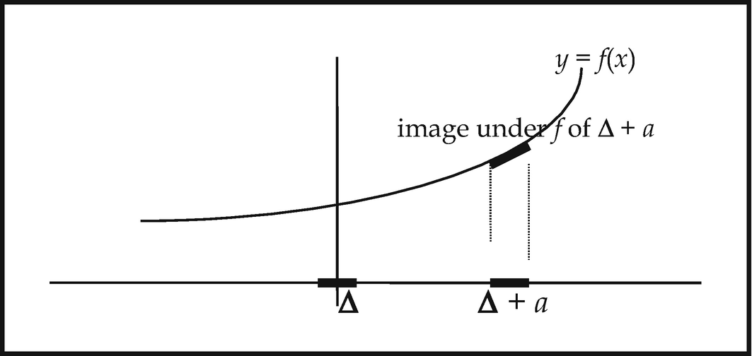
This says that any real-valued function on Δ is affine. If we think of f as a graph in the Cartesian plane, the quantity a measures the displacement, and b the rotation undergone by Δ under the map f.

It follows from the Microaffineness Axiom that any map f: Δ → R ⁿ is of the form

$\upvarepsilon \mapsto \left({a}_1+{b}_1\upvarepsilon, \dots, {a}_n+{b}_n\upvarepsilon \right)$

for unique a ₁, ..., a _n, b ₁, ..., b _n. In particular the image of Δ under f is always a straight line.

The infinitesimal object Δ can be described in number of remarkable ways:

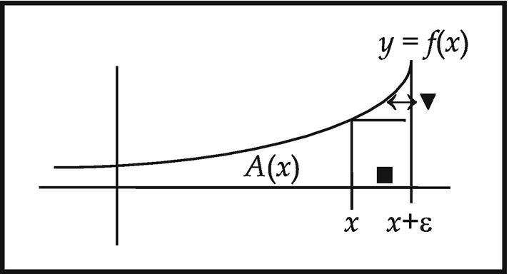
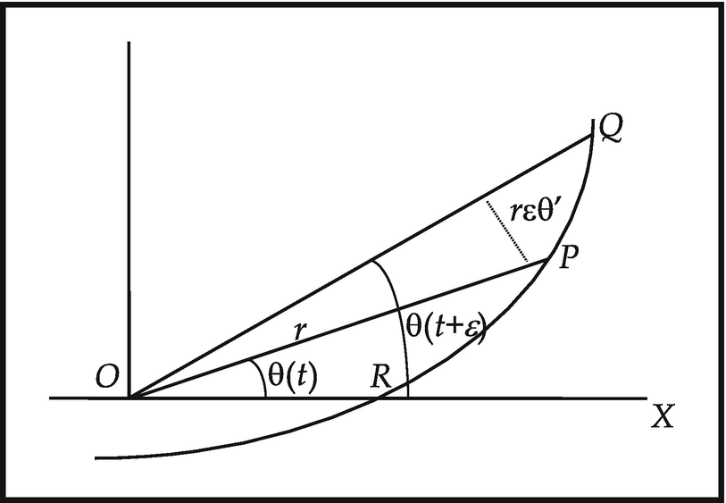
As a generic infinitesimal tangent vector . For consider any curve C in a space S—that is, the image of a segment of R (containing Δ) under a map f into S (Fig. 10.1). Then the image of Δ under f may considered as a short straight line segment lying along C, that is, as part of the tangent to the curve at its contact point actually lying in the curve. Thus curves in S can be considered as infinitesimally straight, or microstraight. This is the Principle of Microstraightness in Space .
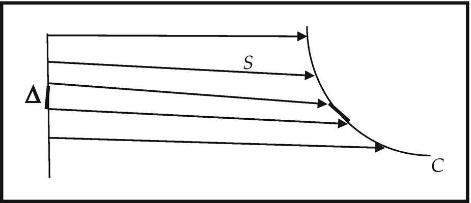Fig. 10.1
Caption
As an intensive magnitude possessing only location and direction, and so which, considered (per impossibile) as an extension, cannot be “bent” or “broken”.
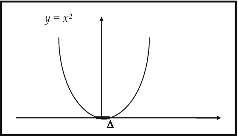
As a domain of nilsquare infinitesimals . For by considering the curve in R × R given by f(x) = x ² , we see that Δ is the intersection of the curve y = x ² with the x-axis⁷ (Fig. 10.2):
Accordingly

../images/474107_1_En_10_Chapter/474107_1_En_10_Fig2_HTML.png — Fig. 10.2
Caption

$\varDelta =\left\{x\in \mathbf{R}:{x}^2=0\right\}.$

We see then that Δ consists of nilsquare infinitesimals , the species of infinitesimal introduced in the seventeenth century by Nieuwentijdt in opposition to Leibniz’s conception.⁸ Such infinitesimals will also be called microquantities. ⁹ As we show below, the axioms we shall introduce for smooth infinitesimal analysis will ensure that Δ is nondegenerate, i.e. does not reduce to {0}, so that Δ may be considered an infinitesimal neighbourhood or microneigbourhood of 0.

As an infinitesimal generator , or microgenerator of spaces . For consider the space Δ ^Δ of self-maps of Δ. It follows from the Microaffineness Axiom that the subspace (Δ ^Δ)₀ of Δ ^Δ consisting of maps vanishing at 0 is isomorphic to R. ¹⁰ Accordingly R, and hence all Euclidean spaces, may be seen as being “generated” by the infinitesimal object Δ.

The space Δ ^Δ is a monoid¹¹ under composition which may be regarded as acting on Δ by evaluation: for f ∈ Δ ^Δ, f ⋅ ε = f(ε). Its subspace (Δ ^Δ)₀ is a submonoid naturally identified as the space of ratios of microquantities. The isomorphism between (Δ ^Δ)₀ and R noted above is easily seen to be an isomorphism of monoids (where R is considered a monoid under its usual multiplication.) It follows that R itself may be regarded as the space of ratios of microquantities. This was essentially the view of Euler , who, as we have seen,¹² regarded (real) numbers as representing the possible results of calculating the ratio 0/0. For this reason Lawvere has suggested that R be called the space of Euler reals. ¹³

As we have said, Δ may be viwed as an intensive magnitude of a certain kind. The microquantities that make up Δ may then be termed intensive quantities. If we think of R as the domain of extensive quantities, then an intensive quantity may be identified as an extensive microquantity , and (by the remarks in the paragraph above) an extensive quantity as the ratio of two intensive quantities.¹⁴

If we think of a smooth world as a model of the natural world, then the Principle of Microstraightness entails not just Leibniz’s Principle of Continuity—that natural processes occur continuously, but also the Principle of Microuniformity, namely, the assertion that any such process may be considered as taking place at a constant rate over any sufficiently small period of time- a Barrovian timelet. For example, if the process is the motion of a particle, the Principle of Microuniformity entails that over an extremely short period the particle undergoes no accelerations. This idea, although rarely explicitly stated, is freely employed in a heuristic capacity in classical mechanics and the theory of differential equations. The virtual equivalence between the Principles of Microuniformity and Microstraightness becomes manifest when natural processes—the motions of bodies, for example, are represented as curves correlating dependent and independent variables. For then, microuniformity of the process is represented by microstraightness of the associated curve.

The Principle of Microstarightness yields an intuitively satisfying account of motion. For it entails that infinitesimal parts of (the curve representing a) motion are not points at which, as Aristotle observed, no motion is detectable—or, indeed, even possible. Rather, infinitesimal parts of the motion are nondegenerate spatial segments just large enough for motion through each to be discernible. On this reckoning a state of motion is to be accorded an intrinsic status, and is not, as Russell claimed, merely to be identified with its result—the successive occupation of a series of distinct positions. Rather, a state of motion is represented by the smoothly varying straight microsegment, the infinitesimal tangent vector , of its associated curve. This straight microsegment may be thought of as an infinitesimal “rigid rod”, just long enough to have a slope—and so, like a speedometer needle, to indicate the presence of motion—but too short to bend, and so also too short to indicate a rate of change of motion.

This analysis may also be applied to the mathematical representation of time. Classically, time is represented as a succession of discrete instants, isolated “nows” at which time has, as it were, stopped. The Principle of Microstraightness , however, suggests that time be instead regarded as a plurality of smoothly overlapping Barrovian timelets each of which may be held to represent a “now” or “specious present” and over which time is, as it were, still passing. This conception of the nature of time is similar to that proposed by Aristotle to refute Zeno’s paradox of the arrow¹⁵; it is also closely related to Peirce’s ideas on time.¹⁶

10.2 Elementary Differential Geometry in a Smooth World

There is a very simple way of constructing the tangent bundle of a space in a smooth world. Let us start with the real line R. Intuitively, the tangent bundle Tan S of a space S is the assemblage of infinitesimally short straight paths in S. In a smooth world such a path may be taken to be a map from the generic tangent vector Δ to S. accordingly the tangent bundle S should be identified with the exponential S ^Δ.

Let us check the compatibility of this definition of Tan S with the usual one in the case of Euclidean spaces R ⁿ. Now R ⁿ has tangent bundle R ⁿ × R ⁿ. But from the Microaffineness Axiom it may be immediately inferred that the map R ^Δ → R × R which assigns to each f ∈ R ^Δ the pair (f(0), slope of f) is an isomorphism. It follows that

$\mathbf{Tan}\left({\mathbf{R}}^n\right)={\left({\mathbf{R}}^n\right)}^{\varDelta}\cong {\left({\mathbf{R}}^{\varDelta}\right)}^n\cong {\left(\mathbf{R}\times \mathbf{R}\right)}^n\cong {\mathbf{R}}^n\times {\mathbf{R}}^n.$

Elements of S ^Δ are called tangent vectors to S. Thus a tangent vector to S at a point p ∈ S is just a map t: Δ → S with t(0) = p. That is, a tangent vector at p is a micropath in S with base point p. The base point map π: TS → S is defined by π(t) = t(0). For p ∈ S, the fibre π⁻¹(p) = Tan _p S is the tangent space to S at p.

Observe that, if we identify each tangent vector with its image in S, then each tangent space to S may be regarded as lying in S. In this sense each smooth space is “infinitesimally flat”.

The assignment S ↦ Tan S = S ^Δ can be turned into a functor in the natural way—the tangent bundle functor . (For f: S → T, Tan f: Tan S → Tan T is defined by (Tan f)t = f _° t for t ∈ Tan S.)

Synthetic differential geometry turns on the fact that the tangent bundle functor is rendered representable: Tan S is “represented” as the space of all maps from some fixed object—in this case Δ)—to S. (Classically, this is impossible.) This in turn simplifies a number of fundamental definitions in differential geometry.

For instance, a vector field on a smooth space S is an assignment of a tangent vector to S at each point in it, that is, a map ξ: S → Tan S = S ^Δ such that ξ(x)(0) = x for all x ∈ S. This means that π _° ξ is the identity on S, so that a vector field is a section of the base point map .

Now we have required that Space be a topos. In particular, for any pair S, T of smooth spaces , Space must also contain their product S × T and their exponential T ^S, the space of all (smooth) maps S → T. These are connected in the following way: for any smooth spaces S, T, U, there is a natural correspondence of maps

$\frac{S\to {T}^U}{S\times U\to T}$

(speaking category-theoretically, the product functor is left adjoint to the exponentiation functor). In the usual function-argument notation, this correspondence is given by:

$\left(f:S\times U\to T\right)\mapsto \left({f}^{\#}:S\to {T}^U\right)\ \mathrm{with}\ {f}^{\#}(s)(u)=f\left(s,u\right)\mathrm{for}\ s\in S,u\in U.$

This gives rise to a correspondence between vector fields on S and what we shall call microflows on S:

$\begin{array}{ll}\underline {\ \xi :S\to {S}^{\varDelta }}& \left(\mathrm{vector}\ \mathrm{fields}\ \mathrm{on}\ S\right)\\ {}{\xi}^{\wedge }:S\times \varDelta \to S& \left(\mathrm{microflows}\ \mathrm{on}\ S\right),\end{array}$

with

${\xi}^{\wedge}\left(x,\upvarepsilon \right)=\xi (x)\left(\upvarepsilon \right).$

Notice that then ξ^{^} (x, 0) = x.

We also get, in turn, a bijective correspondence between microflows on S and micropaths in S ^S with the identity map as base point:

$\begin{array}{cc}\underline {\xi :S\times \varDelta \to S}& \left(\mathrm{microflows}\ \mathrm{on}\ S\right)\\ {}\xi \ast :\varDelta \to {S}^S& \left(\mathrm{micropaths}\ \mathrm{in}\ {S}^S\right),\end{array}$

with

$\xi \ast \left(\upvarepsilon \right)(x)={\xi}^{\wedge}\left(x,\upvarepsilon \right)=\upxi (x)\left(\upvarepsilon \right).$

Thus, in particular,

$\xi \ast (0)(x)=\xi (x)(0)=x,$

so that ξ∗(0) is the identity map on S. Each ξ∗(ε) is a microtransformation of S into itself which is “very close” to the identity map.

Accordingly, in Space , or SDG, vector fields , microflows , and micropaths are equivalent. ¹⁷ Classically, this is a metaphor at best.

There is another remarkable feature of the microgenerator Δ that should be mentioned. First, as Lawvere has emphasized, in smooth categories the tangent bundle functor has an “amazing” right adjoint; that is, for any spaces S, T, there is a natural bijection of maps

$\begin{array}{l}\underline {S^{\varDelta}\to T}\\ {}S\to {T}^{1/\varDelta}\end{array}$

Maps S ^Δ → R are differential forms on S, so the existence of this right adjoint allows differential forms to be represented as maps $S\to {\mathbf{R}}^{\frac{1}{\varDelta }}$ with values in the bigger algebraic structure ${\mathbf{R}}^{\frac{1}{\varDelta }}$ . This feature has led Lawvere to call Δ an “a.t.o.m.”: an “amazingly tiny object model”. Classically, the only objects having this feature are singletons.

10.3 The Calculus in Smooth Infinitesimal Analysis

In the usual development of the calculus, for any differentiable function f on the real line R, y = f(x), it follows from Taylor’s theorem that the increment δy = f(x + δx) – f(x) in y attendant upon an increment δx in x is determined by an equation of the form

$\delta y={f}^{\prime }(x)\delta x+A{\left(\delta x\right)}^2,$

(10.1)

where f′ (x) is the derivative of f(x) and A is a quantity whose value depends on both x and δx. Now if it were possible to take δx a nilsquare infinitesimal or microquantity , then (10.1) would assume the simple form

$f\left(x+\delta x\right)\hbox{--} f(x)=\delta y={f}^{\prime }(x)\delta x.$

(10.2)

In SIA “sufficient” microquantities are present to ensure that Eq. (10.2) holds nontrivially for arbitrary functions f: R → R. (Of course (10.2) holds trivially in standard mathematical analysis because there 0 is the sole microquantity in this sense.) The meaning of the term “nontrivial” here may be explicated in following way. If we replace δx by the letter ε standing for an arbitrary microquantity , (10.2) assumes the form

$f\left(x+\upvarepsilon \right)\hbox{--} f(x)=\upvarepsilon {f}^{\prime }(x).$

(10.3)

Ideally, we want the validity of this equation to be independent of ε, that is, given x, for it to hold for all infinitesimal ε. In that case the derivative f ′(x) may be defined as the unique quantity D such that the equation

$f\left(x+\upvarepsilon \right)\hbox{--} f(x)=\upvarepsilon D$

holds for all microquantities ε.

Setting x = 0 in this equation, we get in particular

$f\left(\upvarepsilon \right)=f(0)+\upvarepsilon D,$

(10.4)

for all ε. Writing, as before, Δ for the set of microquantities, that is,

$\varDelta =\left\{x:x\in \mathbf{R}\wedge {x}^2=0\right\},$

we require that, for any f: Δ → R, there is a unique D ∈ R such that Eq. (10.4) holds for all ε. This says that the graph of f is a straight line passing through (0, f(0)) with slope D. Thus any function on Δ is required to be affine. In SIA this is guaranteed by the Axiom of Microaffiness, as stated above.

If we think of a function y = f(x) as defining a curve, then, for any a, the image under f of the “microinterval” Δ + a obtained by translating Δ to a is straight and coincides with the tangent to the curve at x = a (see Fig. 10.3). In this sense, as in Space , each curve is “microstraight”.¹⁸ This as the Principle of Microstraightness in SIA .

../images/474107_1_En_10_Chapter/474107_1_En_10_Fig3_HTML.png — Fig. 10.3
Caption

From the Microaffiness Axiom we deduce the.

Principle of Microcancellation If εa = εb for all ε, then a = b.

For the premise asserts that the graph of the function g: Δ → R defined by g (ε) = aε has both slope a and slope b: the uniqueness condition in the Microaffineness Axiom then gives a = b. The Principle of Microcancellation supplies the exact sense in which there are “enough” infinitesimals in SIA .

From the Microaffineness Axiom a prercise version of the Principle of Continity can be deduced, namely, that in SIA all functions on R are continuous, in the sense of sending neighbouring points to neighbouring points. (Here two points x, y on R are said to be neighbours if x – y is in Δ, that is, if x and y differ by a microquantity .) To see this, given f: R → R and neighbouring points x, y, note that y = x + ε with ε in Δ, so that

$f(y)\hbox{--} f(x)=f\left(x+\upvarepsilon \right)\hbox{--} f(x)=\upvarepsilon {f}^{\prime }(x).$

But clearly any multiple of a microquantity is also a microquantity, so εf ^′(x) is a microquantity, and the result follows.

Since Eq. (10.3) holds for any f, it also holds for its derivative f ′; it follows that functions in smooth infinitesimal analysis are differentiable arbitrarily many times, thereby justifying the use of the term “smooth”.

Let us derive a basic law of the differential calculus, Leibniz’z product rule:

${(fg)}^{\prime }={f}^{\prime }g+f{g}^{\prime }.$

To do this we compute¹⁹

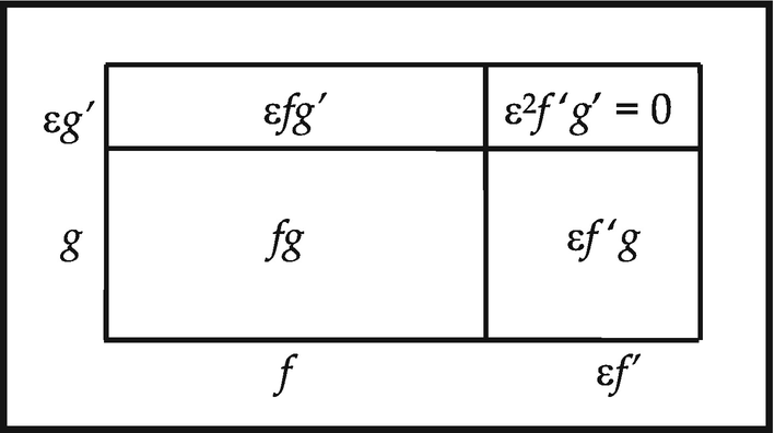
$\begin{array}{lll}(fg)\left(x+\upvarepsilon \right)& =& (fg)(x)+\upvarepsilon {(fg)}^{\prime }(x)=f(x)g(x)+\upvarepsilon {(fg)}^{\prime }(x),\\ {}(fg)\left(x+\upvarepsilon \right)& =& f\left(x+\upvarepsilon \right)g\left(x+\upvarepsilon \right)=\left[f(x)+\upvarepsilon {f}^{\prime }(x)\right]\cdot \left[g(x)+\upvarepsilon\ {g}^{\prime }(x)\right]\\ {}& =& f(x)g(x)+\varepsilon \left({f}^{\prime }g+{fg}^{\hbox{'}}\right)+{\upvarepsilon}^2{f}^{\prime }{g}^{\prime}\\ {}& =& f(x)g(x)+\upvarepsilon \left({f}^{\prime }g+f{g}^{\prime}\right),\end{array}$

since ε² = 0. Therefore ε(fg)^′ = ε(f ^′ g + fg ^′), and the result follows by microcancellation. This calculation is depicted in Fig. 10.4.

../images/474107_1_En_10_Chapter/474107_1_En_10_Fig4_HTML.png — Fig. 10.4
Caption

Next, we derive the Fundamental Theorem of the Calculus (Fig. 10.5).

../images/474107_1_En_10_Chapter/474107_1_En_10_Fig5_HTML.png — Fig. 10.5
Caption

Let J be a closed interval {x: a ≤ x ≤ b} in R and f: J → R; let A(x) be the area under the curve y = f(x) as indicated above. Then, using Eq. (10.3),

$\upvarepsilon {A}^{\prime }(x)=A\left(x+\upvarepsilon \right)\hbox{--} A(x)=\blacksquare +\blacktriangledown =\upvarepsilon f(x)+\blacktriangledown .$

Now by Microstraightnesss ▼ is a triangle²⁰ of area ½ε.ε f ′ (x) = 0. Hence εA′(x) = εf(x), so that, by Microcancellation,

${A}^{\prime }(x)=f(x),$

which is the fundamental theorem of the calculus.

Following Fermat ,²¹ in SIA a stationary point a in R of a function f: R → R is defined to be a point in whose vicinity microvariations fail to change the value of f, that is, for which f(a + ε) = f(a) for all ε. This means that f(a) + εf ′(a) = f(a), so that εf ′(a) = 0 for all ε, from which it follows by microcancellation that f ′(a) = 0. So a stationary point of a function is precisely a point at which the derivative of the function vanishes.

In classical analysis, if the derivative of a function is identically zero, the function is constant. This fact is the source of the following postulate concerning stationary points adopted in SIA:

Constancy Principle . If every point in an interval J is a stationary point of f: J → R (that is, if f ′ is identically 0), then f is constant.

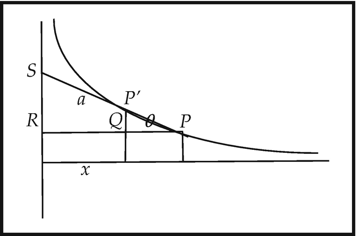
It follows from the Constancy Principle that two functions with identical derivatives differ by at most a constant. Thus if we define an antiderivative of a function f: J → R to be a function g: J → R such that g′ = f, then any function with an antiderivative has a unique antiderivative. This observation, combined with the Principles of Microstraightness and Microcancellation , yields simple derivations of basic equations of mathematics and physics.²² We illustrate the method by deriving the equation of a tractrix.

The tractrix has the property that the length of the tangent to the curve from an arbitrary point on it to the y-axis is constant. It is the curve traced out by an object dragged, under the influence of friction, by a string attached to a pulling point that moves at a right angle to the initial line between the object and the puller.

Referring to Fig. 10.6, let P, P′ be two neighbouring points on the tractrix curve y = y(x) with coordinates (x, y) and (x - ε, y(x - ε)) respectively. Let a be the constant length of the tangent from a point of the curve to the y-axis. Then by Microstraightness the tangent PS to the curve passes thfrough P′. Write L for the length of a line segment L. Then we have

$\underline {P^{\prime }Q}=y\left(x-\upvarepsilon \right)-y(x)=-\upvarepsilon {y}^{\prime}\left(\mathrm{x}\right).$

(∗)

But also, writing θ for the angle RPS, we have.

$\underline {P^{\prime }Q}=\underline{PQ}\;\mathrm{tan}\uptheta =\upvarepsilon \mathrm{tan}\uptheta =\upvarepsilon \underline{RS}/\underline {\mathrm{PR}}=\upvarepsilon {\left({a}^2-{x}^2\right)}^{\frac{1}{2}}/x.$

Equating this with (∗) gives.

$\upvarepsilon {y}^{\prime}\left(\mathrm{x}\right)=-\upvarepsilon {\left({a}^2\hbox{--} {x}^2\right)}^{\frac{1}{2}}/x.$

Using Microcancelletion to cancel ε on both sides of this equation, we get.

${y}^{\prime}\left(\mathrm{x}\right)=-{\left({a}^2\hbox{--} {x}^2\right)}^{\frac{1}{2}}/x.$

(∗∗)

Accordingly y(x) is the antiderivative of the function -(a ² – x ²)^½/x. But the usual computation in the differential calculus (which holds in SIA ) shows that antiderivative to be the function alog[(a + (a ² – x ²)^½)/x)] -(a ² – x ²)^½ . Since, by the Constancy Principle , antiderivatives are unique, it follows that.

$y=a\;\log \left[\left(a+{\left({a}^2\hbox{--} {x}^2\right)}^{\frac{1}{2}}\right)/x\right)\Big]-{\left({a}^2\hbox{--} {x}^2\right)}^{\frac{1}{2}}$

This is the equation of the tracrix.

../images/474107_1_En_10_Chapter/474107_1_En_10_Fig6_HTML.png — Fig. 10.6
Caption

This sort of argument is typical in SIA . The pattern is this. Suppose we want to determine the explicit form of a function f(x). We subject x to a microvariation by adding an infiniresimal ε, and consider the “increment” in f, δf = f(x + ε) – f(x) = εf ′(x). Then we use geometric or other methods “in the small” (i.e. employing microstraightness and the nilsquare propery of ε) to present δf in the form εg(x), where g(x) is an explicit function with explicit antiderivative h. Since εf ′(x) = εg(x), microcancellation gives f ′(x) = g(x). Accordingly f is also an antiderivative of g, and so must be identical with h. This latter function is the explicit form of f.

Put succinctly, the Constancy Principle asserts that “universal infinitesmal (or “local”) constancy implies global constancy”, or “infinitesimal behaviour determines global behaviour” The Constancy Principle brings into sharp focus the difference in SIA between points and infinitesimals. For if in the Constancy Principle one replaces “infinitesimal constancy” by “constancy at a point” the the resulting “Principle” is false because any function whatsoever is constant at every point. But since in SIA all functions on R are microaffine and hence smooth, the Constancy Principle embodies the idea that for such functions local constancy is sufficient for global constancy, that a nonconstant smooth function must be somewhere nonconstant over arbitrarily small intervals.

The Constancy Principle may be seen as furnishing the “missing link” between the infinitesimal and the world “in the large”, the lack of which, as we have already observed, Hermann Weyl believed doomed the idea of infinitesimal, and led to its inevitable replacement by thde limit concept:

[In its struggle with the infinitely small] the limiting process was victorious. For the limit is an indispensable concept, whose importance is not affected by the acceptance or rejection of the infinitely small. But once the limit concept has been grasped, it is seen to render the infinitely small superfluous. Infinitesimal analysis proposes to draw conclusions by integration from the behavior in the infinitely small, which is governed by elementary laws, to the behavior in the large; for instance, from the universal law of attraction for two material “volume elements” to the magnitude of attraction between two arbitrarily shaped bodies with homogeneous or non-homogeneous mass distribution. If the infinitely small is not interpreted ‘potentially’ here, in the sense of the limiting process, then the one has nothing to do with the other, the process in infinitesimal and finite dimensions become independent of each other, the tie which binds them together is cut. ²³

In a smooth world the Constancy Principle reconnects the infinitesimal and the extended. Behaviour “in the large” is completely determined by behaviour “in the infinitely small”.

10.4 The Internal Logic of a Smooth World Is Intuitionistic

The correctness of the Principle of Continuity in SIA induces a subtle, but significant change of logic there: from classical to intuitionistic. For, in the first place, we have only to observe that, if the law of excluded middle held without qualification, then each real number x would either be equal to 0 or unequal to 0, in which case the correlation 0 ↦ 0, x ↦ 1 for x ≠ 0 (the well-known “blip” function) would define a map from the space R of real numbers to the set 2 = {0, 1}; but it is evidently discontinuous, contradicting the Principle of Continuity. From this we see that the Principle of Continuity mplies that the law of excluded middle cannot be universally affirmed in SIA. In fact, this informal argument shows that the statement.

$for\ any\ real\kern0.17em number\ x, either\ x=0\ or\ x\ne 0.$

(∗)

is refutable in SIA .

Here is a rigorous refutation²⁴ 0f (∗) in SIA using the Principle of Microcancellation . To begin with, if x ≠ 0, then x ² ≠ 0, so that, if x ² = 0, then necessarily not x ≠ 0. This means that.

$for\ all\ infinitesimal\ \upvarepsilon, not\ \upvarepsilon \ne 0.$

(∗∗)

Now suppose that (∗) were to hold. Then we would have, for any ε, either ε = 0 or ε ≠ 0. But (∗∗) allows us to eliminate the second alternative, and we infer that, for all ε, ε = 0. This may be written.

$for\ all\ \upvarepsilon, \upvarepsilon .1=\upvarepsilon .0,$

from which we derive by Microcancellation the falsehood 1 = 0. The refutability of (∗) follows.

For simplicity we sgall refer to the refutability of the assertion (∗) as the refutability of the law of excluded middle in SIA .

The Principle of Continuity also implies that propositional functions, or predicates, cannot be taken as being merely “bipolar” in Wittgenstein’s sense, that is, representable in terms of assuming just two “truth values” within the set 2 = {true, false} = {1, 0}. For let Ω be the domain of truth values in a world in which the Principle holds. Then, as usual, for any object X, parts of X correspond to predicates on X, that is “propositional functions” on X, in other words maps X → Ω. Now if X is a (connected) continuum, it presumably does have proper nonempty parts. But there are only two continuous maps X → 2, namely the constant ones corresponding to the whole of X and the empty part of X, because a nonconstant continuous such map on X would yield a “splitting” of X into two nontrivial disconnected pieces. Thus: X has more than two parts; these correspond to maps X → Ω., so there are more than two of these; but there are just two maps X → 2; whence Ω ≠ 2.

It is of interest to recall²⁵ in this connection Peirce’s awareness, even before Brouwer , of the fact that a faithful account of the truly continuous would involve abandoning the unrestricted applicability of the law of excluded middle :

Now if we are to accept the common idea of continuity...we must either say that a continuous line contains no points...or that the law of excluded middle does not hold of these points. The principle of excluded middle applies only to an individual...but places being mere possibilities without actual existence are not individuals.

The prescience shown by Peirce here is all the more remarkable since in SIA the law of excluded middle does, in a certain sense, apply to individuals. This follows from the fact that, despite its failure for arbitrary predicates, the law of excluded middle can be shown to hold in SIA for arbitrary closed sentences. ²⁶ So if P is any predicate and a any particular real number , P(a) ∨ _¬ P(a) will be true. Also for any particular real numbers a, b the statement a = b ∨ a ≠ b holds. Note, however, that in SIA the truth of this last statement for each pair of particular real numbers does not imply the truth of the universal generalization.

$\forall x\in \mathbf{R}\forall y\in \mathbf{R}\;\left(x=y\vee x\ne y\right).$

Indeed, we have seen that this is refutable in SIA : in short, equality on R is undecidable. This may be taken as indicating that the smooth real line is a genuine continuum in being, unlike a discrete set, more than the mere “sum” of its elements.

The “internal” logic of SIA is accordingly not full classical logic. It is, instead, intuitionistic logic , that is, the logic derived from the constructive interpretation of mathematical assertions.²⁷ This “change of logic” is not noticed in the development of basic calculus because there arguments are in the main constructive, proceeding by direct computation.

The refutability of the law of excluded middle in SIA leads to the refutability of an important principle of set theory, the Axiom of Choice . This is the assertion.

(AC) for any family of inhabited²⁸ sets, there is a choice function on , that is, a function f: →∪ for which f(X) ∈ X whenever X ∈ .

Now the law of excluded middle can be derived merely from the very special case of the Axiom of Choice which asserts merelythat any doubleton {U, V} has a choice function. For let p be any proposition, define

$U=\left\{x\in 2:x=0\vee p\right\}\;V=\left\{x\in 2:x=1\vee p\right\}.$

and let f be a choice function on {U, V}. Writing a = f (U), b = f(V), we have a ∈ U, b ∈ V, i.e.,

$\left[a=0\vee p\right]\wedge \left[b=1\vee p\right].$

It follows that

$\left[a=0\wedge b=1\right]\vee p,$

whence

$a\ne b\vee p.$

(∗)

Now clearly

$p\to U=V=2\to a=b,$

whence

$a\ne b\to \neg p,$

But this and (∗) together imply _¬ p ∨ p.

Thus the law of excluded middle is derivable from this special case of the Axiom of Choice . Since the law of excluded middle is refutable in SIA , so equally, then, is AC.

The refutability of the Axiom of Choice in SIA, and hence its incompatibility with the Principle of Continuity which prevails in smooth worlds, is not surprising in view of the Axiom’swell-known “paradoxical” consequences. One of these is the famous Banach-Tarski paradox ²⁹ which asserts that any solid sphere can be decomposed into finitely many pieces which can themselves be reassembled to form two solid spheres each of the same size as the original, or into one solid sphere of any preassigned size. Paradoxical decompositions such as these become possible only when continuous geometric objects are, in Dedekind ’s words,³⁰ “dissolved to atoms ... [through a] frightful, dizzying discontinuity” into discrete sets of points which the axiom of choice then allows to be rearranged in an arbitrary (discontinuous) manner. Such procedures are inadmissible in smooth worlds.

In this connection, it should also be mentioned that the classical intermediate value theorem , often taken as expressing an “intuitively obvious” property of continuous functions , is false in smooth worlds. The intermediate value theorem is the assertion that, for any a, b ∈ R such that a < b, and any continuous f: [a, b] → R such that f(a) < 0 < f(b), there is x ∈[a, b] for which f(x) =0. In fact this fails in SIA even for polynomial functions, as the following informal argument shows. Suppose, for example, that the intermediate value theorem were true in SIA for the polynomial function f(x) = x ³ + tx + u. Then the value of x for which f(x) = 0 would have to depend smoothly on the values of t and u. To be precise, there would have to exist a smooth map g: R ² → R such that

$g{\left(t,u\right)}^3+ tg\left(t,u\right)+u=0.$

A geometric argument can be given to prove that no such smooth map exists.³¹

10.5 Smooth Infinitesimal Analysis as an Axiomatic Theory. Consequences for the Continuum

SIA can be axiomatized as a theory formulated within higher-order intuitionistic logic . Here are the basic axioms of the theory.³²

Axioms for the continuum, or smooth real line R. These include the usual axioms for a commutative ring with unit expressed in terms of two operations + and ., (we usually write xy for x . y) and two distinguished elements 0 ≠ 1.³³ In addition we stipulate that R is an intuitionistic field, i.e., satisfies the following axiom:

$x\ne 0\ \mathrm{implies}\exists y\left( xy=1\right).$

Axioms for the strict order relation < on R. These are:

O1. a < b and b < c implies a < c.
O2. ¬(a < a).
O3. a < b implies a + c < b + c for any c.
O4. a < b and 0 < c implies ac < bc.
O5. either 0 < a or a < 1.
O6. a ≠ b implies a < b or b < a. ³⁴
O7. 0 < x implies ∃y (x = y ²).

Arithmetical Axioms. These govern the set N of Archimedean (or smooth) natural numbers, and read as follows:

1.
N is a cofinal or Archimedean subset of R, i.e. N ⊆ R and ∀x ∈ R ∃n ∈ N x < n.
2.
Peano axioms:

$\begin{array}{l}\begin{array}{c}0\in \mathbf{N}\\ {}\forall x\in \mathbf{R}\left(x\in \mathbf{N}\to x+1\in \mathbf{N}\right)\end{array}\\ {}\forall x\in \mathbf{R}\left(x\in \mathbf{N}\to x+1\ne 0\right)\end{array}$

3.
Restricted Induction scheme. For every formula φ(x) involving just =,∧, ∨, T, ⊥, ∃³⁵

$\upvarphi (0)\kern0.75em \forall x\in \mathbf{N}\left[\upvarphi (x)\to \upvarphi \left(x+1\right)\right]\to \forall x\in N\upvarphi (x).$

Using restricted induction it follows that

N has decidable equality, i.e. ∀x ∈ ∀ y ∈ N(x = y ∨ x ≠ y)
N is linearly ordered, i.e. ∀x ∈ N ∀ y ∈ N(x < y ∨ x = y ∨ y < x).
N satisfies decidable induction: for any formula φ(x),

$\forall x\in \mathbf{N}\left(\upvarphi (x)\vee \neg \upvarphi (x)\right)\to \left[\right[\upvarphi (0)\wedge \forall x\in \mathbf{N}\left(\upvarphi (x)\to \upvarphi \left(x+1\right)\right]\to \forall x\upvarphi (x)\Big].$

The relation ≤ on R is defined by a ≤ b ⇔ ¬b < a. The open interval (a, b) and closed interval [a, b] are defined as usual, viz. (a, b) = {x: a < x < b} and [a, b] = {x: a ≤ x ≤ b}; similarly for half-open, half-closed, and unbounded intervals.

We have written Δ for the subset {x: x ² = 0} of R consisting of (nilsquare) infinitesimals or microquantities. As before, we use the letter ε as a variable ranging over Δ. Δ is subject to the.

Microaffineness Axiom . For any map g: Δ → R there exist unique a, b ∈ R such that, for all ε, we have

$g\left(\upvarepsilon \right)=a+b\upvarepsilon .$

In SIA one also assumes the.

Constancy Principle . If A ⊆ R is any closed interval on R, or R itself, and f: A → R satisfies f(a + ε) = f(a) for all a ∈ A and ε ∈ Δ, then f is constant.

It follows easily from the Microaffineness Axiom that Δ is nondegenerate, i.e. Δ ≠ {0}.³⁶ For if Δ = {0}, then the identity map i: Δ → Δ can be represented as i(ε) = bε for any b, in violation of the uniqueness condition on b.

From the nondegeneracy of Δ we can also (again) refute the law of excluded middle in SIA , more particularly, we can prove.

$\neg \forall \upvarepsilon \left(\upvarepsilon =0\vee \upvarepsilon \ne 0\right).$

(∗)

For we have, for ε ∈ Δ, ε² = 0, whence ¬(ε ≠ 0), and (∗) would give ε = 0. So Δ would be degenerate, contrary to fact. It follows from (∗) that, using x and y as variables ranging over R,

$\neg \forall x\forall y\left(x=y\vee x\ne y\right).$

In a word, the identity relation is undecidable on R.

Call a binary relation S on R stable if it satisfies

$\forall x\forall y\left(\neg \neg xRy\to xRy\right).$

Then the nondegeneracy of Δ implies that, in SIA the equality relation is unstable. For suppose that = were stable . Then, for any ε, it would be the case that ¬ε ≠ 0 → ε =0. But we have already shown above that ¬(ε ≠ 0), so it would follow that ε =0. This being the case for any ε, Δ would be degenerate.

Except for the presence of intuitionistic logic , we note that the algebraic structure on R in SIA differs little from the classical situation. In SIA, R is equipped with the usual addition and multiplication operations under which it is a field. In particular, R satisfies the condition that each x ≠ 0 has a multiplicative inverse. Notice, however, that since in SIA no microquantity (apart from 0 itself) is provably ≠ 0, microquantities are not required to have multiplicative inverses (a requirement which would lead to inconsistency). From a strictly algebraic standpoint, R in SIA differs from its classical counterpart only in being required to satisfy the Principle of Microcancellation .

The situation is otherwise, however, as regards the order structure of R in SIA. Since microquantities do not have multiplicative inverses, and R is an intuitionistic field, it must be the case that ∀ε¬(ε ≠ 0), whence

$\forall \upvarepsilon \neg \left(\upvarepsilon <0\vee \neg \upvarepsilon >0\right),$

or equivalently

$\forall \upvarepsilon \left(\upvarepsilon \le 0\wedge \upvarepsilon \ge 0\right).$

It follows easily from this and the nondegeneracy of Δ that

$\neg \forall x\forall y\left(x<y\vee y<x\vee x=y\right).$

In other words the order relation < on R in SIA fails to satisfy the trichotomy law ; it is a partial, rather than a total ordering.

The axioms of SIA entail that R differs in certain key respects from its counterpart in constructive analysis CA .³⁷ For example, in CA the equality relation is stable , while we have ashown above that in SIA iit is unstable. Also in CA the ordering relation < satisfies

$\neg \left(x<y\vee y<x\right)\to x=y;$

(∗)

and this is incompatible with the axioms of SIA . For (∗) implies.

$\forall x\neg \left(x<0\vee 0<x\right)\to x=0.$

(∗∗)

But in SIA it is easy to derive

$\forall x\in \varDelta \kern0.5em \neg \left(x<0\vee 0<x\right),$

and this, together with (∗∗), would give Δ = {0}, contradicting the nondegeneracy of Δ.

In CA the object Δ is degenerate while the nondegeneracy of Δ in SIA is one of its characteristic features.

Axiom O6 of SIA, together with the transitivity and irreflexivity of <, implies that < is stable . This may be seen as follows. Suppose ¬¬a < b. Then certainly a ≠ b, since a = b → ¬a < b by irreflexivity. Therefore a < b or b < a. The second disjunct together with ¬¬a < b and transitivity gives ¬¬a < a, which contradicts ¬a < a. Accordingly we are left with a < b. Hence < is stable . But the stability of < cannot be deduced in CA .³⁸

10.6 Cohesiveness of the Continuum and Its Subsets in SIA

In oclassical analysis the continuum and its closed intervals are connected in the sense that they cannot be split into two nonempty subsets neither of which contains a limit point of the other. In SIA the Constancy Principle ensures that these have the vastly stronger property of cohesiveness, ³⁹ that is, they cannot be split into two disjoint nonempty subsets in any way whatsoever. This is clearly equivalent to saying that any map A → {0, 1} is constant.

To see this, let A be R or any closed interval, and suppose A = U ∪ V with U ∩ V = ∅. Define f: A → {0, 1} by f(x) = 1 if x ∈ U, f(x) = 0 if x ∈ V. We claim that f is constant. For we have

$\left(f(x)=0\ \mathrm{or}\ f(x)=1\right)\kern0.5em \&\kern0.5em \left(f\left(x+\upvarepsilon \right)=0\ \mathrm{or}\ f\left(x+\upvarepsilon \right)=1\right).$

This gives four possibilities:

(i)
f(x) = 0 & f(x + ε) = 0
(ii)
f(x) = 0 & f(x + ε) = 1
(iii)
f(x) = 1 & f(x + ε) = 0
(iv)
f(x) = 1 & f(x + ε) = 1

Possibilities (ii) and (iii) may be ruled out because f is continuous. This leaves (i) and (iv), in either of which f(x) = f(x + ε). So f is locally, and hence globally, constant, that is, constantly 1 or 0. In the first case V = ∅, and in the second case U = ∅ .

From the cohesiveness of closed intervals it can be inferred⁴⁰ that in SIA all intervals in R are cohesive.

In SIA cohesive subsets of R correspond, grosso modo, to connected subsets of ℝ in classical analysis, that is, to intervals. This is borne out by the fact that any puncturing of R is decomposable, for it follows immediately from Axiom O6 that

$\mathbf{R}\hbox{--} \left\{a\right\}=\left\{x:x>a\right\}\cup \left\{x:x<a\right\}.$

The set Q of (smooth) rational numbers is defined as usual to be the set of all fractions of the form m/n with m, n ∈ N , n ≠ 0. The fact that N is cofinal in R ensures that Q is dense in R .

The set R – Q of irrational numbers is decomposable as

$\mathbf{R}\hbox{--} \mathbf{Q}=\left[\left\{x:x>0\right\}\hbox{--} \mathbf{Q}\right]\cup \left[\left\{x:x<0\right\}\hbox{--} \mathbf{Q}\right\}.$

This is in sharp contrast with the situation in intuitionistic analysis that is, CA augmented by Kripke’s scheme , Brouwer ’s Continuity Principle, and bar induction . For we have observed⁴¹ that in intuitionistic analysis not only is any puncturing of R cohesive, but that this is even the case for the irrational numbers. This would seem to indicate that in some sense the continuum in SIA is considerably less “syrupy”⁴² than its counterpart in SIA.

It can also be shown that the various infinitesimal neighbourhoods of 0 are cohesive⁴³ (see Fig. 10.7). The cohesiveness of the first of these infinitesimal neighbourhoods, Δ itself, can be established as follows. Suppose f: Δ → {0, 1}. Then by Microaffineness there are unique a, b ∈ R such that f(ε) = a + bε for all ε. Now a = f(0) = 0 or 1; if a = 0, then bε = f(ε) = 0 or 1, and clearly bε ≠ 1. So in this case f(ε) = 0 for all ε. If on the other hand a = 1, then 1 + bε = f(ε) = 0 or 1; but 1 + bε = 0 would impl bε = −1 which is again impossible. So in this case f(ε) = 1 for all ε. Therefore f is constant and Δ cohesive.

../images/474107_1_En_10_Chapter/474107_1_En_10_Fig7_HTML.png — Fig. 10.7
Caption

In SIA nilpotent infinitesimals are defined to be the members of the sets.

${\boldsymbol{\Delta}}_k=\left\{x\in \mathbf{R}:{{x^k}^{+}}^1=0\right\},$

for k = 1, 2, ..., each of which may be considered an infinitesimal neighbourhood of 0. These are subject to the.

Micropolynomiality Principle . For any k ≥ 1 and any g: Δ _k → R, there exist unique a, b ₁, ..., b _k ∈ R such that for all δ ∈ Δ _k we have.

$g\left(\updelta \right)=a+{b}_1\updelta +{b}_2{\updelta}^2+\dots +{\mathrm{b}}_{\mathrm{k}}\;{\updelta}^{\mathrm{k}}.$

Micropolynomiality implies that no Δ _k coincides with {0}.

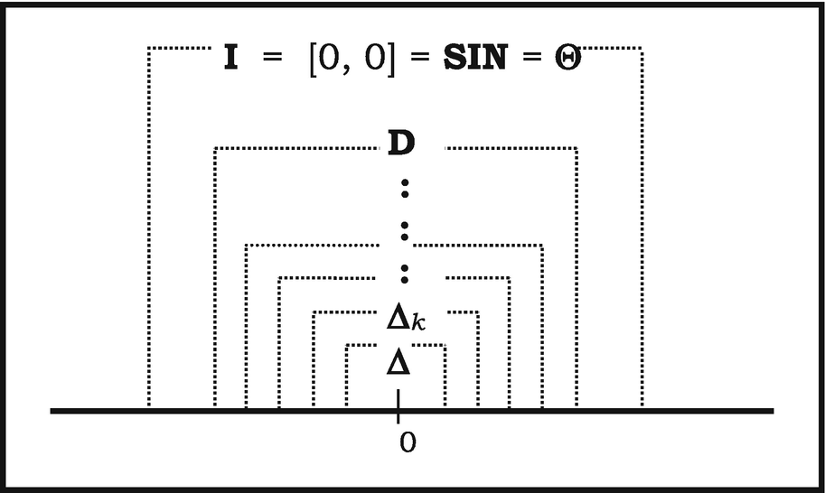
An argument similar to that establishing the cohesiveness of Δ does the same for each Δ _k. Thus let f: Δ _k → {0, 1}; Micropolynomiality implies the existence of a, b ₁, ..., b _k ∈ R such that f(δ) = a + ζ(δ), where ζ(δ) = b ₁δ + b ₂δ² + ... + b _kδ^k. Notice that ζ(δ) ∈ Δ _k, that is, ζ(δ) is nilpotent. Now a = f(0) = 0 or 1; if a = 0 then ζ(δ) = f(δ) = 0 or 1, but since ζ(δ) is nilpotent it cannot =1. Accordingly in this case f(δ) = 0 for all δ ∈ Δ _k. If on the other hand a = 1, then 1 + ζ(δ) = f(δ) = 0 or 1, but 1 + ζ(δ) = 0 would imply ζ(δ) = −1 which is again impossible. Accordingly f is constant and Δ cohesive.

The union D of all the Δ _k is the set of nilpotent infinitesimals , another infinitesimal neighbourhood of 0. The cohesiveness of D follows readily from that of each Δ _k.

The next infinitesimal neighbourhood of 0 is [0, 0], which, as a closed interval, is cohesive. It is easily shown that [0, 0] includes D, so that it does not coincide with {0}.

It can be shown that [0, 0] coincides with the set Θ of noninvertible elements of R, as well as with the sets

$\mathbf{SIN}=\left\{x\in \mathbf{R}:\forall n\in \mathbf{N}\left(-\frac{1}{n+1}<x<\frac{1}{n+1}\right)\right\}.$

of strict infinitesimals , as well as the set

$\mathbf{I}=\left\{x\in \mathbf{R}:\neg x\ne 0\right\}$

of elements of R indistinguishable from 0. I is an ideal, in fact a maximal ideal in the ring R.

Finally, we observe that the sequence of infinitesimal neighbourhoods of 0 generates a strictly ascending sequence of decomposable subsets containing R – {0}, namely:

$\mathbf{R}-\left\{0\right\}\subset \left(\mathbf{R}-\left\{0\right\}\right)\cup \left\{0\right\}\subset \left(\mathbf{R}-\left\{0\right\}\right)\cup {\varDelta}_1\subset \left(\mathbf{R}-\left\{0\right\}\right)\cup {\varDelta}_2\subset \dots \left(\mathbf{R}-\left\{0\right\}\right)\cup \mathbf{D}\subset \left(\mathbf{R}-\left\{0\right\}\right)\cup \left[0,0\right].$

10.7 Comparing the Smooth and Dedekind Real Lines in SIA

A Dedekind real is a pair (U, V) ∈ ../images/474107_1_En_10_Chapter/474107_1_En_10_Figb_HTML.gif

Q ×

Q ⁴⁴ satisfying the conditions:

$\exists x\exists y\left(x\in U\wedge y\in V\right)$

$U\cap V=\varnothing$

$\forall x\left(x\in U\leftrightarrow \exists y\in U.x<y\right)$

$\forall x\left(x\in V\leftrightarrow \exists y\in V.y<x\right)$

$\forall x\forall y\left(x<y\to x\in U\vee y\in V\right).$

The set R _d of Dedekind reals can be turned into an ordered ring.⁴⁵ This ring is always constructively complete , that is, satisfies the condition: Let A be an inhabited subset of R _d that is bounded above. Then sup A exists if and only if for all x, y ∈ R _d with x < y, either y is an upper bound for A or there exists a ∈ A with x < a. (A real number b is called a supremum , or least upper bound, of A if it is an upper bound for A and if for each ε > 0 there exists x ∈ A with x > b – ε.)

Although R _d is constructively complete, it is not conditionally complete in the classical sense because of the failure of the logical law ¬p ∨ ¬¬p. ⁴⁶ But R _d shares some features of the constructive reals not possessed by R, e.g.

$\neg \neg x=y\to x=y$

$x\le y\wedge y\le x\to x=y$

${x}^n=0\to x=0.$

There is a natural order preserving homomorphism φ: R → R _d given by.

$\upvarphi (r)={\left(\left\{q\in \mathbf{Q}:q<r\right\},\left\{q\in \mathbf{Q}:q>r\right\}\right)}^{\prime }$

This is injective on Q, and embeds Q as the rational numbers in R _d . Moreover, the kernel of φ coincides with the ideal I of strict infinitesimals in R, so φ induces an embedding of the quotient ring R/I into R _d . R/I is R shorn of its nilpotent infinitesimals : it is both an intuitionistic field and an integral domain , that is, satisfies

$\forall x\left(x\ne 0\to x\ is\ invertible\right)\kern1.00em \forall x\forall y\left[ xy=0\to x=0\vee y=0\right].$

It can be shown that φ is surjective—so that R/I ≅ R _d—precisely when R is constructively complete in the sense above. In that event R _d is both an intuitionistic field and an integral domain, properties that the ring of Dedekind reals in a topos does not always possess.

In any model of SIA the usual open interval topology can be defined on R _d. It can be shown⁴⁷ that with this topology R _d is always connected in the sense that it cannot be partitioned into two disjoint inhabited open subsets. In SIA R _d actually inherits a stronger cohesiveness property from R. To see this, call a subset X of a set A detachable ⁴⁸ if there is a subset Y of A such that X ∩ Y = ∅, X ∪ Y = A. Now we can show that, if X is a detachable subset of R _d, then φ [R] ⊆ X or X ∩ φ[R] = ∅ . For suppose X ⊆ R _d detachable and define f: R _d → 2 by f(x) = 1 if x ∈ X, f(x) = 0 if x ∉ X. Then f ° φ: R → 2 must be constant since R is cohesive. If f ° φ is constantly 1, then φ[R] ⊆ X; if constantly 0, then A ∩ φ[R] = ∅. It follows easily that if φ is surjective then R _d is itself cohesive.

10.8 Nonstandard Analysis in SIA

In certain models of SIA the system of natural numbers possesses some intriguing features which make it possible to introduce another type of infinitesimal—the so-called invertible infinitesimals —resembling those of nonstandard analysis , whose presence engenders yet another infinitesimal neighbourhood of 0 properly containing all those introduced above.

We recall that the set N of smooth natural numbers is required to satisfy not the full principle of mathematical induction for arbitrary properties but only the weaker restricted induction scheme. This raises the possibility that N may not coincide with the set ℕ of standard natural numbers, which is defined to be the smallest subset of R containing 0 and closed under the operation of adding 1. Now, models of SIA have been constructed⁴⁹ in which ℕ is a proper subset of N; accordingly the members of N – ℕ may be considered nonstandard integers. Multiplicative inverses of nonstandard integers are infinitesimals, but, being themselves invertible, they are of a different type from the (necessarily noninvertible) nilpotent infinitesimals which are basic to SIA.

Proceeding formally, we define the set ℕ of standard natural numbers to be the intersection of all inductive subsets of N, i.e.,

$\mathrm{\mathbb{N}}=\left\{n\in \mathbf{N}:\forall X\subseteq \mathbf{N}\left[0\in X\wedge \forall m\left(m\in X\to m+1\in X\right)\to n\in X\right]\right\}$

ℕ evidently satisfies full induction :

$\forall X\subseteq \mathbf{N}\left[0\in X\wedge \forall m\left(m\in X\to m+1\in X\right)\to X=\mathbf{N}\right].$

The space of infinitesimals is the set

$\mathbf{IN}=\left\{x\in \mathbf{R}:\forall n\in \mathrm{\mathbb{N}}\right(-1/\left(n+1\right)<x<1/\left(n+1\right)\Big\}.$

This is the largest infinitesimal neighbourhood of zero in SIA : it contains the space Θ of noninvertible infinitesimals as well as the space of invertible or Robinsonian infinitesimals

$\mathrm{I}=\left\{x\in \mathbf{IN}:x\ is\ invertible\right\}.$

As inverses of “infinitely large” reals (i.e. reals r satisfying ∀n ∈ ℕ . n < r ∨ ∀n ∈ ℕ . r < −n) invertible infinitesimals are the counterparts in SIA of the infinitesimals of nonstandard analysis .⁵⁰ Invertible infinitesimals are strictly larger than their noninvertible cousins in that

$\forall x\forall y\left[x\in \Theta \wedge y\in \mathrm{I}\ y>0\to x<y\right].$

To assert the existence of invertible infinitesimals is to assert that I is inhabited⁵¹: this is equivalent to asserting that the set N – ℕ of nonstandard integers is inhabited, or equivalently, that the following holds:

$\exists n\in \mathbf{N}\forall m\in \mathrm{\mathbb{N}}m<n.$

When this condition is satisfied, as it is in certain models of SIA , we shall say that nonstandard integers, or invertible infinitesimals , are present. Notice that while it is perfectly consistent to assert the presence of invertible infinitesimals, i.e., that I be inhabited, it is inconsistent to assert the “presence” of nonzero noninvertible infinitesimals, i.e. that Θ – {0} be inhabited.⁵²

One may also postulate the condition

$\forall n\in \mathbf{N}\left[\forall x\in \mathbf{N}\hbox{--} \mathrm{\mathbb{N}}\left(x>n\right)\to n\in \mathrm{\mathbb{N}}\right],$

i.e. “a natural number which is smaller than all nonstandard natural numbers must be standard”. This is in fact equivalent to the condition that ℕ be a stable subset of N, i.e. N – (N – ℕ) = ℕ. Assuming that nonstandard integers are present, this latter may be understood as asserting that as many as possible of these are present.

In the presence of invertible infinitesimals R _d is a nonstandard model of the reals lacking nilpotent elements. The passage via φ from R to R _d eliminates the nilpotent elements but preserves invertible infinitesimals. When φ is onto, R _d is a cohesive nonstandard model of the reals.

Within R we have the subring of accessible reals

${\mathbf{R}}_{\mathbf{acc}}=\left\{x\in \mathbf{R}:\exists n\in \mathrm{\mathbb{N}}\left(\hbox{--} n<x<n\right)\right\},$

in which I is an ideal. Since each open interval in R is cohesive, R _acc satisfies the condition of being an inhabited set which includes, for each pair x, y of its members, a cohesive subset I for which {x, y} ⊆ I. It follows from this that R _acc is cohesive.

Within R _d the subring of finite reals may be identified:

${\mathbf{R}}_{\mathbf{fin}}=\left\{x\in {\mathbf{R}}_{\mathbf{d}}:\exists n\in \mathrm{\mathbb{N}}\left(\hbox{--} n<x<n\right)\right\}.$

Clearly φ carries R _acc into R _fin. Since R _acc is cohesive, R _fin inherits a cohesiveness property analogous to that possessed by R _d, namely, if X is a detachable subset of R _fin, then φ[R _acc] ⊆ X or X ∩ φ[R _acc] = ∅.

We observe that R _fin can only be a detachable subset of R _d when N = ℕ, or equivalently, when R _acc and R coincide, or to put it another way, when no invertible infinitesimals are present. For if R _fin is detachable in R _d, then, as above, either φ[R] ⊆ R _fin, or R _fin ∩ φ[R] = ∅. The latter being obviously false, it follows that φ[R] ⊆ R _fin. But then φ[N] ⊆ R _fin ∩ φ[N] = φ[ℕ], whence N = ℕ.

10.9 Contrasting Nonstandard Analysis with Smooth Infinitesimal Analysis

Smooth infinitesimal analysis shares with nonstandard analysis the feature that continuity is represented by the idea of “preservation of infinitesimal closeness”. Nevertheless, there are a number of differences between the two approaches:

In models of SIA , only smooth maps between objects are present. In models of NSA, all set-theoretically definable maps (including, in particular, discontinuous ones) appear.
The logic of SIA is intuitionistic, making possible the nondegeneracy of the infinitesimal neigbourhoods Δ, D and SIN. The logic of NSA is classical,⁵³ causing all these neighbourhoods to collaose to {0}.
In SIA , all curves are microstraight, and closed curves infinilateral polygons . Nothing resembling this is present in NSA.
The nilpotency of the infinitesimals of SIA reduces the differential calculus to simple algebra. In NSA the use of infinitesimals is a disguised form of the classical limit method.
The hyperreal line in NSA is obtained by augmenting the classical real line with infinitesimals (and infinite numbers), while the smooth real line R comes already equipped with infinitesimals.
In any model of NSA, the hyperreal line ℝ^★ has exactly the same set-theoretically expressible properties as does the classical real line: in particular ℝ^★ is an archimedean field in the sense of that model. This means that the infinitesimals (and infinite numbers) of NSA are not intrinsically so in the sense of the model in which they “live”, but only relative to the “standard” model with which the construction began. That is, speaking figuratively, an inhabitant of a model of NSA would be unable to detect the presence of infinitesimals or infinite numbers in ℝ^★. This contrasts with SIA in two respects. First, in models of SIA containing invertible infinitesimals , the real line is nonarchimedean with respect to the set of standard natural numbers, which is itself an object of the model. In other words, the presence of (invertible) infinitesimals and infinite numbers would be perfectly detectable by an inhabitant of the model. And secondly, the characteristic property of nilpotency possessed by the microquantities of a model of SIA is an intrinsic property, perfectly identifiable within the model. In NSA the hyperreals have precisely the same algebraic properties as do the classical real numbers , but the smooth reals in SIA do not.

The differences between NSA and SIA arise because the former is essentially a theory of infinitesimal numbers designed to provide a succinct formulation of the limit concept, while the latter is, by contrast, a theory of infinitesimal geometric objects, designed to provide an intrinsic formulation of the concept of differentiability.

10.10 Smooth Infinitesimal Analysis and Physics

In the past physicists showed no hesitation in employing infinitesimal methods,⁵⁴ the use of which in turn relied on the implicit assumption that the (physical) world is smooth, or at least that the maps encountered there are differentiable as many times as needed. For this reason smooth infinitesimal analysis provides an ideal framework for the rigorous derivation of results in classical physics.⁵⁵ We present two here.

First, we derive the equation of continuity for fluids, whose original derivation by Euler was outlined in Chap. 3. The derivation in SIA will follow Euler’s very closely, but the use of nilsquare infinitesimals and the Microcancellation Axiom will render the argument entirely rigorous.

Before we begin we require a few observations on partial derivatives in SIA. Given a function f: R ⁿ → R of n variables x ₁, ..., x _n, the partial derivative $\frac{\partial f}{\partial {x}_i}$ is defined as usual to be the derivative of the function f (a ₁, ..., x _i, ..., a _n) obtained by fixing the values of all the variables apart from x _i. In that case, for an arbitrary microquantity ε, we have

$f\left({x}_1,\dots, {x}_i+\upvarepsilon, \dots, {x}_n\right)+\upvarepsilon \frac{\partial f}{\partial {x}_i}\left({x}_1,\dots, {x}_n\right).$

(10.5)

Using the fact that ε² = 0, it is then easily shown that

$f\left({x}_1+{a}_1\upvarepsilon, \dots, {x}_n+{a}_n\upvarepsilon \right)=f\left({x}_1,\dots, {x}_n\right)+\upvarepsilon \sum \limits_{i=1}^n{a}_i\frac{\partial f}{\partial {x}_i}\left({x}_1,\dots, {x}_n\right).$

(10.6)

These equations are pivotal in deriving the equation of continuity. Here we are given a inviscid fluid of varying density flowing smoothly in space . At any point O = (x, y, z) in the fluid and at any time t, the fluid’s density ρ and the components u, v, w of the fluid’s velocity are given as functions of x, y, z, t. Following Euler , we consider the elementary volume element E —a microparallelepiped—with origin O and edges OA, OB, BC of microlengths ε, η, ζ and so of mass εηζρ:

Fluid flow during the microtime τ transforms the volume element E into the microparallelepiped E′ (Fig. 10.8) with vertices O′, A′, B′, C′. We first calculate the length of the side O′A′. Now, using (10.5), the rate at which A is moving away from O in the x-direction is

$u\left(x+\upvarepsilon, y,z,t\right)-u\left(x,y,z,t\right)=\upvarepsilon \frac{\partial u}{\partial x}.$

The change in length of OA during the microtime τ is thus $\upvarepsilon \uptau \frac{\partial u}{\partial x},$ so that the length of O’A’ is $\upvarepsilon +\upvarepsilon \uptau \frac{\partial u}{\partial x}=\upvarepsilon \left(1+\uptau \frac{\partial u}{\partial x}\right).$ Similarly, the lengths of O′B′ and O′C′ are, respectively,

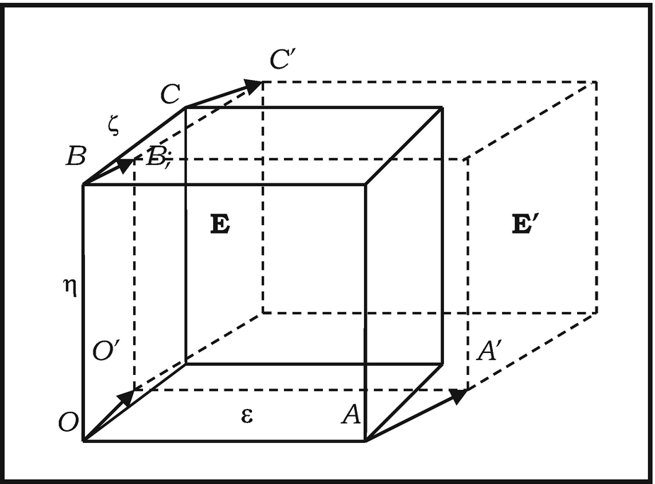
../images/474107_1_En_10_Chapter/474107_1_En_10_Fig8_HTML.png — Fig. 10.8
Caption

$\upeta \left(1+\uptau \frac{\partial v}{\partial y}\right),\upzeta \left(1+\uptau \frac{\partial w}{\partial z}\right).$

The volume of E′ is the product of these three quantities, which, using the fact that τ² = 0, comes out as

$\upvarepsilon \upeta \upzeta \left[1+\uptau \left(\frac{\partial u}{\partial x}+\frac{\partial v}{\partial y}+\frac{\partial w}{\partial z}\right)\right].$

(10.7)

Since the coordinates of O′ are (x + uτ, y + vτ, z + wτ), the fluid density ρ’ there at timet + τ is, using (10.6),

$\uprho +\uptau \left(\frac{\mathrm{\partial \uprho }}{\partial t}+u\frac{\mathrm{\partial \uprho }}{\partial x}+v\frac{\mathrm{\partial \uprho }}{\partial y}+w\frac{\mathrm{\partial \uprho }}{\partial z}\right).$

(10.8)

The mass of E′ is then the product of (10.7) and (10.8), which, again using the fact that that τ² = 0, comes out as

$\upvarepsilon \upeta \upzeta \uprho +\upvarepsilon \upeta \upzeta \uptau \left(\frac{\mathrm{\partial \uprho }}{\partial t}+\uprho \frac{\partial u}{\partial x}+\uprho \frac{\partial v}{\partial y}+\uprho \frac{\partial w}{\partial z}+u\frac{\mathrm{\partial \uprho }}{\partial x}+v\frac{\mathrm{\partial \uprho }}{\partial y}+w\frac{\mathrm{\partial \uprho }}{\partial z}\right).$

(10.9)

Now by the principle of conservation of mass, the masses of the fluid in E and E′ are the same, so equating the mass εηζρ of E to the mass of E′ given by (10.9) yields

$\upvarepsilon \upeta \upzeta \uptau \left(\frac{\mathrm{\partial \uprho }}{\partial t}+\uprho \frac{\partial u}{\partial x}+\uprho \frac{\partial v}{\partial y}+\uprho \frac{\partial w}{\partial z}+u\frac{\mathrm{\partial \uprho }}{\partial x}+v\frac{\mathrm{\partial \uprho }}{\partial y}+w\frac{\mathrm{\partial \uprho }}{\partial z}\right)=0.$

Microcancellation gives

$\frac{\mathrm{\partial \uprho }}{\partial t}+\uprho \frac{\partial u}{\partial x}+\uprho \frac{\partial v}{\partial y}+\uprho \frac{\partial w}{\partial z}+u\frac{\mathrm{\partial \uprho }}{\partial x}+v\frac{\mathrm{\partial \uprho }}{\partial y}+w\frac{\mathrm{\partial \uprho }}{\partial z}=0,$

i.e.,

$\frac{\mathrm{\partial \uprho }}{\partial t}+\frac{\partial }{\partial x}\left(\uprho u\right)+\frac{\partial }{\partial y}\left(\uprho v\right)+\frac{\partial }{\partial z}\left(\uprho w\right)=0,$

Euler’s equation of continuity .

Next, we derive the Kepler-Newton areal law of motion under a central force . We suppose that a particle executes plane motion under the influence of a force directed towards some fixed point O. If P is a point on the particle’s trajectory with coordinates x, y, we write r for the length of the line PO and θ for the angle that it makes with the x-axis OX. Let A be the area of the sector ORP, where R is the point of intersection of the trajectory with OX. We regard x, y, r, θ as functions of a time variable t: thus

$x=x(t),y=y(t),r=r(t),\uptheta =\uptheta (t),A=A(t).$

Now let Q be a point on the trajectory at which the time variable has value t + ε, with ε in Δ (Fig. 10.9). Then by Microstraightness the sector OPQ is a triangle of base r(t + ε) = r + εr’ and height

../images/474107_1_En_10_Chapter/474107_1_En_10_Fig9_HTML.png — Fig. 10.9
Caption

$r\ \sin \left[\uptheta \left(t+\upvarepsilon \right)-\uptheta (t)\right]=r\ \sin\ \upvarepsilon {\uptheta}^{\prime }=r\upvarepsilon {\uptheta}^{\prime }{.}^{56}$

The area of OPQ is accordingly

$2\ \mathrm{base}\times \mathrm{height}=2\left(r+\upvarepsilon {r}^{\prime}\right)r\upvarepsilon {\uptheta}^{\prime }=2\left({r}^2\upvarepsilon {\uptheta}^{\prime }+{\upvarepsilon}^2r{r}^{\prime }{\uptheta}^{\prime}\right)=2{r}^2\upvarepsilon {\uptheta}^{\prime }.$

Therefore

$\upvarepsilon {A}^{\prime }(t)=A\left(t+\upvarepsilon \right)\hbox{--} A(t)= area\ OPQ=2\upvarepsilon {r}^2{\uptheta}^{\prime },$

so that, cancelling ε,

${A}^{\prime }(t)=2{r}^2{\uptheta}^{\prime }.$

(∗)

Now let H = H(t) be the acceleration towards O induced by the force. Resolving the acceleration along and normal to OX, we have

${x}^{{\prime\prime} }=H\ \mathrm{cos}\uptheta \kern1.5em {y}^{{\prime\prime} }=H\ \mathrm{sin}\uptheta .$

Also x = r cosθ, y = r sinθ. Hence

$y{x}^{{\prime\prime} }= Hy\ \mathrm{cos}\uptheta = Hr\ \sin\ \uptheta\ \cos\ q\kern2em x{y}^{{\prime\prime} }= Hx\ \mathrm{sin}\uptheta = Hr\ \mathrm{sin}\uptheta\ \mathrm{cos}\uptheta,$

from which we infer that

${\left(x{y}^{\prime}\hbox{--} y{x}^{\prime}\right)}^{\prime }=x{y}^{{\prime\prime}}\hbox{--} y{x}^{{\prime\prime} }=0.$

Hence

$x{y}^{\prime}\hbox{--} y{x}^{\prime }=k,$

(∗∗)

where k is a constant.

Finally, from x = r cosθ, y = r sinθ, it follows in the usual way that

$x{y}^{\prime}\hbox{--} y{x}^{\prime }={r}^2{\uptheta}^{\prime },$

and hence, by (∗∗) and (∗), that

${A}^{\prime }(t)=2k.$

Assuming A(0) = 0, we conclude that

Thus the radius vector joining the body to the point of origin sweeps out equal areas in equal times (Kepler’s law).

Here is an appropriate place to remark on an intriguing use of infinitesimals in Einstein’s celebrated 1905 paper On the Electrodynamics of Moving Bodies, ⁵⁶ in which the special theory of relativity is first formulated. In deriving the Lorentz transformations from the principle of the constancy of the velocity of light Einstein obtains the following equation for the time coordinate τ(x’, y, z, t) of a moving frame⁵⁷:

$\frac{1}{2}\left[\uptau \left(0,0,0,t\right)+\uptau \left(0,0,0,t+\frac{x^{\prime }}{c-v}+\frac{x^{\prime }}{c+v}\right)\right]=\uptau \left({x}^{\prime },0,0,t+\frac{x^{\prime }}{c-v}\right).$

(10.10)

He continues:

Hence, if x’ be chosen infinitesimally small,

$\frac{1}{2}\left(\frac{1}{c-v}+\frac{1}{c+v}\right)\frac{\mathrm{\partial \uptau }}{\partial t}=\frac{\mathrm{\partial \uptau }}{\partial {x}^{\prime }}+\frac{1}{c-v}\frac{\mathrm{\partial \uptau }}{\partial t},$

(10.11)

$\frac{\mathrm{\partial \uptau }}{\partial {x}^{\prime }}+\frac{v}{c^2-{v}^2}\frac{\mathrm{\partial \uptau }}{\partial t}=0.$

Now the derivation of Equation ( _10.11 ) from equation ( _10.10 ) can be simply and rigorously carried out in SIA by choosing x′ to be a microquantity ε. For then ( _10.10 ) becomes

$\frac{1}{2}\left[\uptau \left(0,0,0,t\right)+\uptau \left(0,0,0,t+\upvarepsilon \left(\frac{1}{c-v}+\frac{1}{c+v}\right)\right)\right]=\uptau \left(\upvarepsilon, 0,0,t+\frac{\upvarepsilon}{c-v}\right).$

From this we get, using equation (1) above,

$\uptau \left(0,0,0,t\right)+\frac{1}{2}\upvarepsilon \left(\frac{1}{c-v}+\frac{1}{c+v}\right)\frac{\mathrm{\partial \uptau }}{\partial t}=\uptau \left(0,0,0,t\right)+\upvarepsilon \left(\frac{\mathrm{\partial \uptau }}{\partial {x}^{\prime }}+\frac{1}{c-v}\frac{\mathrm{\partial \uptau }}{\partial t}\right).$

$\frac{1}{2}\upvarepsilon \left(\frac{1}{c-v}+\frac{1}{c+v}\right)\frac{\mathrm{\partial \uptau }}{\partial t}=\upvarepsilon \left(\frac{\mathrm{\partial \uptau }}{\partial {x}^{\prime }}+\frac{1}{c-v}\frac{\mathrm{\partial \uptau }}{\partial t}\right),$

and (ii) follows by microcancellation.

Spacetime metrics have some arresting properties in SIA . In a spacetime the metric can be written in the form.

${ds}^2=\Sigma {g}_{\upmu \mathrm{v}}{dx}_{\upmu}{dx}_{v\kern1.75em }\upmu, v=1,2,3,4.$

(∗)

In the classical setting (∗) is in fact an abbreviation for an equation involving derivatives and the “differentials” ds and dx _μ are not really quantities at all. What form does this equation take in SIA ? Notice that the “differentials” cannot be taken as microquantities since all the squared terms would vanish. But the equation does have a very natural form in terms of microquantities. Here is an informal way of obtaining it.

We think of the dx _μ as being multiples k _μ e of some small quantity e. Then (∗) becomes

${ds}^2={e}^2\Sigma {g}_{\upmu \mathrm{v}}{k}_{\upmu}{k}_v,$

so that

$\mathrm{d}s=e\sqrt{\Sigma {g}_{\upmu \mathrm{v}}{k}_{\upmu}{k}_v}.$

Now replace e by a microquantity ε. Then we obtain the metric relation: in SIA

$\mathrm{d}s=\upvarepsilon \sqrt{\Sigma {g}_{\upmu \mathrm{v}}{k}_{\upmu}{k}_v}.$

This tells us that the “infinitesimal distance ” ds between a point P with coordinates (x ₁, x ₂, x ₃, x ₄) and an infinitesimally near point Q with coordinate (x ₁ + k ₁ε, x ₂ + k ₂ε, x ₃ + k ₃ε, x ₄ + k ₄ε) is $\upvarepsilon \sqrt{\Sigma {g}_{\upmu \mathrm{v}}{k}_{\upmu}{k}_v}$ . Here a curious situation arises. For when the “infinitesimal interval” ds between P and Q is timelike (or lightlike), the quantity Σg _μv k _μ k _vis nonnegative, so that its square root is a real number . In this case ds may be written as εd, where d is a real number. On the other hand, if ds is spacelike, then Σg _μv k _μ k _vis negative, so that its square root is imaginary. In this case, then, ds assumes the form iεd, where d is a real number (and, of course $\mathrm{i}=\sqrt{-1}$ ). On comparing these we see that, if we take ε as the “infinitesimal unit” for measuring infinitesimal timelike distances, then iε serves as the “imaginary infinitesimal unit” for measuring infinitesimal spacelike distances .

For purposes of illustration (Fig. 10.10), let us restrict the spacetime to two dimensions (x, t), and assume that the metric takes the simple form ds² = dt ² – dx ². The infinitesimal light cone at a point P divides the infinitesimal neighbourhood at P into a timelike region T and a spacelike region S bounded by the null lines l and l′ respectively (see Fig. 10.9). If we take P as origin of coordinates , a typical point Q in this neighbourhood will have coordinates (aε, bε) with a and b real numbers: if | b| > |a|, Q lies in T; if a = b, P lies on l or l′; if |a| < |b|, P lies in S. If we write $d=\sqrt{\mid {a}^2-{b}^2\mid }$ , then in the first case, the infinitesimal distance between P and Q is εd, in the second, it is 0, and in the third it is iεd.

../images/474107_1_En_10_Chapter/474107_1_En_10_Fig10_HTML.png — Fig. 10.10
Caption

Minkowski introduced “ict” to replace the “t” coordinate so as to make the metric of relativistic spacetime positive definite. This was purely a matter of formal convenience and was later rejected by (general) relativists.⁵⁸ In conventional physics one never works with nilpotent quantities so it is always possible to replace formal imaginaries by their (negative) squares. But spacetime theory in SIA forces one to use imaginary units, since, infinitesimally, one can’t “square oneself out of trouble”. This being the case, it would seem that, infinitesimally, Misner, Thorne and Wheeler’s⁵⁹ dictum Farewell to ict needs to be replaced by

$Vale\ ict, ave\ \mathrm{i}\upvarepsilon !$

To quote Misner, Thorne and Wheeler again,

Another danger in curved spacetime is the temptation to regard ... the tangent space as lying in spacetime itself. This practice can be useful for heuristic purposes but is incompatible with complete mathematical precision. ⁶⁰

The consistency of SIA shows that, on the contrary, yielding to this temptation is compatible with complete mathematical precision: there tangent spaces may indeed be regarded as lying in spacetime itself.

We conclude this section with a speculation. Observe that the microobject Δ is “tiny” in the order-theoretic sense. For, using ε, η, as variables ranging over Δ, it is easily seen that that.

$\forall \upvarepsilon \forall \upeta \neg \left(\upvarepsilon <\upeta \vee \upeta <\upvarepsilon \right).$

(∗)

whence

$\forall \upvarepsilon \forall \upeta \left(\upvarepsilon \le \upeta \wedge \upeta \le \upvarepsilon \right).$

In particular, the members of Δ are all simultaneously ≤ 0 and ≤0 but cannot (because of the nondegeneracy of Δ) be shown to coincide with zero.

In his book Just Six Numbers ⁶¹ the astrophysicist Martin Rees comments on the microstructure of space and time, and the possibility of developing a theory of quantum gravity. In particular he says:

Some theorists are more willing to speculate than others. But even the boldest acknowledge the “ Planck scales ” as an ultimate barrier. We cannot measure distances smaller than the Planck length [about 10 ¹⁹ times smaller than a proton]. We cannot distinguish two events (or even decide which came first) when the time interval between them is less than the Planck time (about 10 ^–43 seconds).

On this account, Planck scales seem very similar in certain respects to Δ. In particular, the sentence (∗) above seems to be an exact embodiment of the idea that we cannot decide of two “events” in Δ which came first; in fact it makes the stronger assertion that actually neither comes “first”.

Could Δ serve as a suitable model for “Planck scales ”? While Δ is unquestionably small enough to play the role, it inhabits a domain in which everything is smooth and continuous, while Planck scales live in the quantum world which, if not outright discrete, is far from being universally continuous. So if Planck scales could indeed be modelled by microneighbourhoods in SIA , then one might begin to suspect that the quantum microworld, the Planck regime—smaller, in Rees’s words, “than atoms by just as much as atoms are smaller than stars”—is not, like the world of atoms, discrete, but instead continuous like the world of stars. This would be a major victory for the Continuous in its long struggle with the Discrete.

10.11 Relating Sets and Smooth Spaces

Considerable light is shed on the nineteenth century arithmetization , or set-theorization, of analysis by examining the relationship that exists between Space and the category Set of sets.⁶²

While the law of excluded middle holds in Set, we have seen that it fails in Space. In particular the identity relation on the smooth real line R in Space is not decidable , that is, with variables x, y over R,

$\neg \forall x\forall y\left[x=y\vee x\ne y\right].$

This may be understood as saying that elements of R cannot always be fully distinguished; R is amorphous in some degree . While R contains “well-distinguished” points such as 0, 1, π, etc., it cannot, unlike a discrete set, actually be made up of these.

Now, as we have seen, this is precisely the view that most mathematicians and philosophers took of the geometric line, and of continua generally, before the nineteenth century set-theorization of analysis. This suggests that we view the objects of Space as representing continua as they were conceived before that process took place.⁶³ It is also reasonable to take the smooth maps in Space as representing the functions between continua actually recognized by pre-nineteenth century mathematicians, since these were, before the emergence of the notion of a function as an arbitrary correspondence, mostly smooth in any case. The category Space accordingly provides a working “model” of the pre-set-theoretic mathematics of continua.

As we know, the view that a mathematical continuum cannot be composed of points began to change in the nineteenth century, giving way to the arithmetization of analysis and the emergence of a set-theoretic, or discrete, account of the continuum. In effect, this meant the displacement of Space by Set as the locus of activity in mathematical analysis. Let us investigate the relation between the two.

First, certain objects in Space may be identified as “set-like”. These are the discrete spaces S which consist of well-distinguished elements in that the law of excluded middle in the form

$\forall x\forall y\left[x=y\vee x\ne y\right]$

holds with variables x, y over S. (It is easily shown, for example that the space N of natural numbers is discrete.) Since every object in Set is discrete in this sense, discrete spaces are the counterparts, in Space, of sets.⁶⁴

Next, recall that each topological space or manifold has an underlying set of elements or points; we want to extend this idea to a space as an object of Space. What should we mean by a point of a space? The natural response is to define a point of a space S to be a map (in Space) from the terminal object (one-point space) 1 to S. We think of points as being the smallest possible nonempty spaces, so it is natural to stipulate that Space satisffy the

Points Axiom . Each space is either empty or has points.

It follows from this axion that, for any points p, q of a space, either p = q or p ≠ q. In other words, as Aristotle asserted, points either coincide or are totally separate. Clearly 0 is then the only point of Δ.

To ensure that each space has an underlying set of points we introduce the

Discrete Subspace Axiom . Each space S has a unique discrete subspace ΓS such that every point of S is in ΓS.

The space ΓS is called the set of points of the space S. It is the “arithmetized” or “atomized” version of S. ΓS may be thought of as the set obtained from S by removing the “glue” binding the points of S together. Notice that ΓΔ = {0}.

These new axioms (together with those of SIA ) suffice to ensure that each space S has an underlying set of points and each map between spaces induces an underlying function between the corresponding sets of points. But “the underlying sets and functions are far too weakly axiomatized to supply foundations for geometry”.⁶⁵ In the case of the smooth real line R, for example, the stated axioms ensure only that its underlying set of points ΓR = ℝ is a field, nothing more than a discrete algebraic structure. For ℝ to provide an adequate surrogate for R, it is necessary to capture the concept of convergence , of capital importance to the arithmetical account of the continuum. Since the amorphousness of R undermines the uniqueness of the limit required by the theory of convergence, whatever axioms are introduced to ensure that the usual convergence criteria introduced by Cauchy are satisfied, they must of necessity be formulated for ℝ rather than R. This fact helps to explain why “Cauchy’s theory of convergence led towards set-theoretic as opposed to geometric foundations.”⁶⁶

We have seen that, following Weierstrass’s lead, Cantor and Dedekind laboured to formulate an independent characterization of ℝ as a discrete set of real numbers . Working as they did “only with discrete collections, using the law of excluded middle ”^, ⁶⁷ their efforts can be seen as taking place in Set rather than Space. Each provided a definition of ℝ as an ordered field, both postulating in addition that “this represented the set of points on the geometric line with [its] arithmetic and order relation.”⁶⁸ In effect, they “defined ℝ within Set and added an axiom ΓR = ℝ plus others for arithmetic and order.”⁶⁹

We turn next to the space R ^R of maps from R to R in Space. We need to distinguish carefully between Γ(R ^R), the set of functions corresponding to smooth maps from R to R, and ΓR ^ΓR = ℝ^ℝ, the set of arbitrary functions from ℝ to ℝ. Clearly, however, Γ(R ^R) ⊆ ℝ^ℝ; in fact, it can be shown that every function in Γ(R ^R) has derivatives of all orders.

The set Γ(R ^R) includes all the real-valued functions known to eighteenth century mathematics, in particular, the polynomial, trigonometric, and exponential functions and all functions obtained by composing these. Γ(R ^R) may be said to represent functions of “the well-behaved form with which mathematicians [of the day] were familiar”.⁷⁰ But the work of Fourier on trigonometric series in the early nineteenth century stimulated mathematicians to begin to admit as “functions” not of that well-behaved form, that is, functions which are clearly not in Γ(R ^R).⁷¹ but which we would today recognize as being in ℝ^ℝ. This development provided a further motive for the development of an independent theory of ℝ, so also assisting in leading analysis away from Space to Set .

The upshot was that “the [geometric] line came to be defined as ℝ with additional structure [and] smooth maps were defined to be functions with derivatives of all orders .” Set theory came to dominate analysis, and, eventually, geometry as well. In the process, as we have seen, infinitesimals fell by the wayside,⁷² not to be returned to active duty for another three-quarters of a century. Even more lamentably,

the disappearance of infinitesimals is only a symptom of a deeper loss . The independent reality of spaces and maps almost disappeared from mathematical consciousness as everything was reduced to sets. ⁷³

It is fortunate that today, through category theory and intuiutionistic logic, the means for reviving the geometric vision are at hand.

Bibliography

Bell, J.L. 1998. A Primer of Infinitesimal Analysis. Cambridge: Cambridge University Press. Second edition 2oo8.
———. 2001. In The Continuum in Smooth Infinitesimal Analysis, ed. Peter Schuster, Ulrich Berger, and Horst Osswald, 19–24. Dordrecht: Kluwer Academic Publishers.
Boyer, C. 1968. A History of Mathematics. Hoboken: Wiley.
Bridges, D., and F. Richman. 1987. Varieties of Constructive Mathematics. Cambridge: Cambridge University Press.Crossref
Busemann, H. 1955. The Geometry of Geodesics. New York: Academic.
Dummett, M. 1977. Elements of Intuitionism. Oxford: Clarendon Press.
Einstein, A., et al. 1952. The Principle of Relativity : a Collection of Original Memoirs on the Special and General Theory of Relativity. Trans. Perrett and Jeffrey. Dover. Reprint of 1923 Methuen edition.
Johnstone, P.T. 1977. Topos Theory. London: Academic.
Kock, A. 1981. Synthetic Differential Geometry. Cambridge: Cambridge University Press.
Lawvere, F.W. 2011. Euler’s continuum functorially vindicated. In Vintage Enthusiasms: Essays in Honour of John L. Bell, ed. D. Devidi, P. Clark, and M. Hallett. Dordrecht: Springer.
McLarty, C. 1988. Defining sets as sets of points of spaces. Journal of Philosophical Logic 17: 75–90.Crossref
———. 1992. Elementary Categories, Elementary Toposes. Oxford: Oxford University Press.
Misner, C., K. Thorne, and J. Wheeler. 1972. Gravitation. San Francisco: Freeman.
Moerdijk, I., and G.E. Reyes. 1991. Models for Smooth Infinitesimal Analysis. New York: Springer.Crossref
Palmgren, E. 1998. Developments in constructive nonstandard analysis. The Bulletin of Symbolic Logic 4: 233–272.Crossref
Rees, M. 2001. Just Six Numbers: The Deep Forces that Shape the Universe. New York: Basic Books.
Spivak, M. 1975. A Comprehensive Introduction to Differential Geometry. Houston: Publish or Perish Press.
Wagon, S. 1993. The Banach-Tarski Paradox. Cambridge: Cambridge University Press.
Weyl, H. 1949. Philosophy of Mathematics and Natural Science. Princeton: Princeton University Press. (An expanded Engish version of Philosophie der Mathematik und Naturwissenschaft, Leibniz Verlag, 1927.).Crossref
———. 1950. Space-Time-Matter. Trans. Brose, H. Dover. (English translation of Raum, Zeit, Materie, Springer, 1918.)

Footnotes

Busemann (1955).

An Incredible Shrinking Man(ifold), no less.

It is this deficiency that makes the construction of the tangent bundle in Man something of a headache: see Spivak (1975).

That is, differentiable arbitrarily many times

See Chap. 7.

Also known as the Kock-Lawvere axiom after its formulators, Anders Kock and F. W. Lawvere .

This feature of SIA brings to mind Protagoras’s claim (as reported by Aristotle (in Metaphysics III, 2) that “the circle touches the ruler not at a point, but along a line.”

See Chap. 2. It should be pointed out, however, that Nieuwentijdt’s infinitesimals differ from those of SIA in that that the product of any two of the former vanishes, while this is not the case for the latter.

We shall use letters ε, η, ζ to denote arbitrary microquantities.

This can be seen by noting that for any f ∈ R ₀, the Mcroaffineness Axiom ensures that there is a unique b ∈ R for which f(ε) = bε for all ε, and conversely each b ∈ R yields the map ε ↦ bε in R ₀.

A monoid is a multiplicative system (not necessarily commutative) with an identity element.

See Chap. 3.

Lawvere (2011).

This would seem to be consonant with Hermann Cohen’s conception of the infinitesimal as mentioned at the end of Chap. 4.

See Chap. 1.

See Chap. 5.

Note that, with the appropriate choice of maps , each of these constitute the objects of a further topos, the topos of first-order differential structures over objects in S.

And closed curves can be treated as infinilateral polygons , as they were by Galileo and Leibniz .

What follows is surely the prettiest demonstration of the product rule ever devised. Leibniz would have found it delightful.

▼ is in fact the characteristic triangle of seventeenth century analysis (see Chap. 2). As will be seen, in SIA its area reduces to zero.

See Chap. 2.

See Bell (1998).

Weyl (1949) 44–5. Yet we also recall Weyl’s observation:

The principle of gaining knowledge of the external world from the behaviour of its infinitesimal parts is the mainspring of the theory of knowledge in infinitesimal physics as in Riemann’s geometry, and, indeed, the mainspring of all the eminent work of Riemann (Weyl 1950, p. 92).

We givde another refutation of (∗) below.

See Chap. 5.

To be precise, this condition can be shown to hold in a number of models of SIA , See McLarty (1988).

See Chap. 9.

A set is said to be inhabited if it can be constructively shown to have a member. In intuitionistic logic this is a stronger condition than the assertion that the set be nonempty.

See Wagon (1993).

See Chap. 4.

Moerdijk and Reyes (1991), Remark VII.2.14.

Moerdijk and Reyes (1991)

Here a ≠ b stands for ¬a = b.

It should be pointed out that axiom 6 is omitted in some presentations of SIA , e.g. those in Kock (1981) and McLarty (1992).

Here, T, ⊥ are symbols denoting, respectively, the true and the false.

It should be noted that, while Δ does not reduce to {0}, nevertheless 0 is the only explicitly nameable element of Δ. For it is easily seen to be inconsistent to assert that Δ actually contains an element ≠ 0.

See Chap. 9.

In CA , the stability of < can be shown to entail, for certain predicates A, the corresponding instance of Markov’s Principle, namely

$\forall x\left(A(x)\vee \neg A(x)\right)\wedge \neg \forall x\neg A(x)\to \exists xA(x).$

Markov’s principle is not generally accepted in constructive analysis . See Dummett (1977) and Bridges and Richman (1987).

See Appendix A.

Bell (2001).

Chap. 9.

It should be emphasized that this phenomenon is a consequence of axiom O6: it cannot necessarily be affirmed in versions of SIA not including this axiom.

Notice that in CA all of these infinitesimal objects are degenerate. This makes it difficult to formulate a satisfactory theory of infinitesimals in any extension of CA , in particular, in intuitionistic analysis .

Here ../images/474107_1_En_10_Chapter/474107_1_En_10_Figb_HTML.gif A is the power set of a set A.

See Johnstone (1977). In the topos Shv(X) of sheaves over a topological space X, R _d is the sheaf of continuous real-valued functions on open subsets of X.

The failure of this law in SIA follows immediately from the cohesiveness of R by considering the predicate x ≠ 0. As originally shown by Johnstone, conditional completeness of R _d is actually equivalent to this logical law ¬p ∨ ¬¬p: in Shv(X), the law holds iff X is extremally disconnected, that is, the closure of every open set is open.

L. Stout, Topological properties of the real numbers object in a topos. Cahiers Topologie Géom. Différentielle 17, no. 3, (1976), pp. 295-326.

It is easily shown that a subset X of a set A is detachable if and only if the property of being a member of X is decidable , that is, if ∀x∈A(x ∈ X or x ∉ X).

See Moerdijk and Reyes (1991).

IN may accordingly be seen as accommodating both the invertible infinitesimals of Leibniz and the noninvertible nilsquare infinitesimals of Nieuwentijdt .

Recall that a set is A is inhabited if it is nonempty in the strong sense of actually possessing an element, as opposed to the constructively weaker sense of the assertion that it is empty being refutable.

On the other hand it follows from the nondegeneracy of Δ that it is also inconsistent to assert that Θ reduces to {0}.

It should be pointed out, however, that constructive versions of NSA have been developed. See Palmgren (1998).

In this connection we recall, for the last time, the words of Hermann Weyl :

The principle of gaining knowledge of the external world from the behaviour of its infinitesimal parts is the mainspring of the theory of knowledge in infinitesimal physics as in Riemann’s geometry and, indeed, the mainspring of all the eminent work of Riemann (1922, p. 92).

Hilbert declared set theory to be “Cantor’s Paradise”; In the same spirit, SIA could be dubbed “Riemann’s Paradise”. The one, the Paradise of the Discrete; the other, the Paradise of the Continuous.

A number of these are derived in Bell (1998).

Reprinted in English translation in Einstein et al. (1952). It should be noted, however, that in subsequent presentations of special relativity Einstein avoided the use of infinitesimals

Here x’ is simply a symbol for the x-coordinate of the moving frame, not to be confused with the derivative of x.

See, for example Box 2.1 of Misner et al. (1972).

See footnote immediately above.

Op. cit., p. 205.

Ress (2001).

My account here is based on McLarty’s illuminating paper (1988).

In this spirit, we may take the microobjects in Space to represent the diverse theories of infinitesimals that were still in place before set theory swept them away.

As mentioned in McLarty (1988), it can be shown that, in the presence of the axioms for SIA augmented by the two additional axioms introduced below, discrete spaces together with the maps between them form a category which satisfies the system of axioms characterizing the category Set . In this sense Set may be seen as the result of “imposing” the law of excluded middle on the objects of Space , or more precisely, of discarding those objects of Space which fail to satisfy that law. McLarty mentions another method of obtaining Set from Space, that of passing to double-negation sheaves.

McLarty (1988), p. 83.

Op. cit., p. 84

Ibid.

Op. cit., p. 85.

Ibid.

Boyer (1968), p. 600.

For example, Dirichlet’s function r: R → R defined by r(x) =1 for x rational and r(x) = 0 for x irrational.

In the passage from Space to Set , nonzero infinitesimals sink without trace, since the application of Γ reduces microobjects such as Δ to singletons such as {0}.

McLarty (1988), p. 87.

10. Smooth Infinitesimal Analysis/Synthetic Differential Geometry

10.1 Smooth Worlds

10.2 Elementary Differential Geometry in a Smooth World

10.3 The Calculus in Smooth Infinitesimal Analysis

10.4 The Internal Logic of a Smooth World Is Intuitionistic

10.5 Smooth Infinitesimal Analysis as an Axiomatic Theory. Consequences for the Continuum

10.6 Cohesiveness of the Continuum and Its Subsets in SIA

10.7 Comparing the Smooth and Dedekind Real Lines in SIA

10.8 Nonstandard Analysis in SIA

10.9 Contrasting Nonstandard Analysis with Smooth Infinitesimal Analysis

10.10 Smooth Infinitesimal Analysis and Physics

10.11 Relating Sets and Smooth Spaces