
Again, the expression on page F-40 assumes that switches are able to pipeline packet transmission at the packet level.
Following the method presented previously, we can estimate the best-case upper bound for effective bandwidth by finding the narrowest section of the end-to-end network pipe. Focusing on the internal network portion of that pipe, network bandwidth is determined by the blocking properties of the topology. Non-blocking behavior can be achieved only by providing many alternative paths between every source-destination pair, leading to an aggregate network bandwidth that is many times higher than the aggregate network injection or reception bandwidth. This is quite costly. As this solution usually is prohibitively expensive, most networks have different degrees of blocking, which reduces the utilization of the aggregate bandwidth provided by the topology. This, too, is costly but not in terms of performance.
The amount of blocking in a network depends on its topology and the traffic distribution. Assuming the bisection bandwidth, BWBisection, of a topology is implementable (as typically is the case), it can be used as a constant measure of the maximum degree of blocking in a network. In the ideal case, the network always achieves full bisection bandwidth irrespective of the traffic behavior, thus transferring the bottlenecking point to the injection or reception links. However, as packets destined to locations in the other half of the network necessarily must cross the bisection links, those links pose as potential bottleneck links—potentially reducing the network bandwidth to below full bisection bandwidth. Fortunately, not all of the traffic must cross the network bisection, allowing more of the aggregate network bandwidth provided by the topology to be utilized. Also, network topologies with a higher number of bisection links tend to have less blocking as more alternative paths are possible to reach destinations and, hence, a higher percentage of the aggregate network bandwidth can be utilized. If only a fraction of the traffic must cross the network bisection, as captured by a bisection traffic fraction parameter γ (0 < γ ≤ 1), the network pipe at the bisection is, effectively, widened by the reciprocal of that fraction, assuming a traffic distribution that loads the bisection links at least as heavily, on average, as other network links. This defines the upper limit on achievable network bandwidth, BWNetwork:

Accordingly, the expression for effective bandwidth becomes the following when network topology is taken into consideration:

It is important to note that γ depends heavily on the traffic patterns generated by applications. It is a measured quantity or calculated from detailed traffic analysis.
Example
A common communication pattern in scientific programs is to have nearest neighbor elements of a two-dimensional array to communicate in a given direction. This pattern is sometimes called NEWS communication, standing for north, east, west, and south—the directions on a compass. Map an 8 × 8 array of elements one-to-one onto 64 end node devices interconnected in the following topologies: bus, ring, 2D mesh, 2D torus, hypercube, fully connected, and fat tree. How long does it take in the best case for each node to send one message to its northern neighbor and one to its eastern neighbor, assuming packets are allowed to use any minimal path provided by the topology? What is the corresponding effective bandwidth? Ignore elements that have no northern or eastern neighbors. To simplify the analysis, assume that all networks experience unit packet transport time for each network hop—that is, TLinkProp, Tr, Ta, Ts, and packet transmission time for each hop sum to one. Also assume the delay through injection links is included in this unit time, and sending/receiving overhead is null.
Answer
This communication pattern requires us to send 2 × (64 − 8) or 112 total packets—that is, 56 packets in each of the two communication phases: northward and eastward. The number of hops suffered by packets depends on the topology. Communication between sources and destinations are one-to-one, so σ is 100%. The injection and reception bandwidth cap the effective bandwidth to a maximum of 64 BW units (even though the communication pattern requires only 56 BW units). However, this maximum may get scaled down by the achievable network bandwidth, which is determined by the bisection bandwidth and the fraction of traffic crossing it, γ, both of which are topology dependent. Here are the various cases:
 Bus—The mapping of the 8 × 8 array elements to nodes makes no difference for the bus as all nodes are equally distant at one hop away. However, the 112 transfers are done sequentially, taking a total of 112 time units. The bisection bandwidth is 1, and γ is 100%. Thus, effective bandwidth is only 1 BW unit.
- Ring—Assume the first row of the array is mapped to nodes 0 to 7, the second row to nodes 8 to 15, and so on. It takes just one time unit for all nodes simultaneously to send to their eastern neighbor (i.e., a transfer from node i to node i + 1). With this mapping, the northern neighbor for each node is exactly eight hops away so it takes eight time units, which also is done in parallel for all nodes. Total communication time is, therefore, 9 time units. The bisection bandwidth is 2 bidirectional links (assuming a bidirectional ring), which is less than the full bisection bandwidth of 32 bidirectional links. For eastward communication, because only 2 of the eastward 56 packets must cross the bisection in the worst case, the bisection links do not pose as bottlenecks. For northward communication, 8 of the 56 packets must cross the two bisection links, yielding a γ of 10/112 = 8.93%. Thus, the network bandwidth is 2/.0893 = 22.4 BW units. This limits the effective bandwidth at 22.4 BW units as well, which is less than half the bandwidth required by the communication pattern.
- 2D mesh—There are eight rows and eight columns in our grid of 64 nodes, which is a perfect match to the NEWS communication. It takes a total of just 2 time units for all nodes to send simultaneously to their northern neighbors followed by simultaneous communication to their eastern neighbors. The bisection bandwidth is 8 bidirectional links, which is less than full bisection bandwidth. However, the perfect matching of this nearest neighbor communication pattern on this topology allows the maximum effective bandwidth to be achieved regardless. For eastward communication, 8 of the 56 packets must cross the bisection in the worst case, which does not exceed the bisection bandwidth. None of the northward communications crosses the same network bisection, yielding a γ of 8/112 = 7.14% and a network bandwidth of 8/0.0714 = 112 BW units. The effective bandwidth is, therefore, limited by the communication pattern at 56 BW units as opposed to the mesh network.
- 2D torus—Wrap-around links of the torus are not used for this communication pattern, so the torus has the same mapping and performance as the mesh.
- Hypercube—Assume elements in each row are mapped to the same location within the eight 3-cubes comprising the hypercube such that consecutive row elements are mapped to nodes only one hop away. Northern neighbors can be similarly mapped to nodes only one hop away in an orthogonal dimension. Thus, the communication pattern takes just 2 time units. The hypercube provides full bisection bandwidth of 32 links, but at most only 8 of the 112 packets must cross the bisection. Thus, effective bandwidth is limited only by the communication pattern to be 56 BW units, not by the hypercube network.
- Fully connected—Here, nodes are equally distant at one hop away, regardless of the mapping. Parallel transfer of packets in both the northern and eastern directions would take only 1 time unit if the injection and reception links could source and sink two packets at a time. As this is not the case, 2 time units are required. Effective bandwidth is limited by the communication pattern at 56 BW units, so the 1024 network bisection links largely go underutilized.
- Fat tree—Assume the same mapping of elements to nodes as is done for the ring and the use of switches with eight bidirectional ports. This allows simultaneous communication to eastern neighbors that takes at most three hops and, therefore, 3 time units through the three bidirectional stages interconnecting the eight nodes in each of the eight groups of nodes. The northern neighbor for each node resides in the adjacent group of eight nodes, which requires five hops, or 5 time units. Thus, the total time required on the fat tree is 8 time units. The fat tree provides full bisection bandwidth, so in the worst case of half the traffic needing to cross the bisection, an effective bandwidth of 56 BW units (as limited by the communication pattern and not by the fattree network) is achieved when packets are continually injected.
The above example should not lead one to the wrong conclusion that meshes are just as good as tori, hypercubes, fat trees, and other networks with higher bisection bandwidth. A number of simplifications that benefit low-bisection networks were assumed to ease the analysis. In practice, packets typically are larger than the link width and occupy links for many more than just one network cycle. Also, many communication patterns do not map so cleanly to the 2D mesh network topology; instead, usually they are more global and irregular in nature. These and other factors combine to increase the chances of packets blocking in low-bisection networks, increasing latency and reducing effective bandwidth.
To put this discussion on topologies into further perspective, Figure F.16 lists various attributes of topologies used in commercial high-performance computers.

F.5 Network Routing, Arbitration, and Switching
Routing, arbitration, and switching are performed at every switch along a packet’s path in a switched media network, no matter what the network topology. Numerous interesting techniques for accomplishing these network functions have been proposed in the literature. In this section, we focus on describing a representative set of approaches used in commercial systems for the more commonly used network topologies. Their impact on performance is also highlighted.
Routing
The routing algorithm defines which network path, or paths, are allowed for each packet. Ideally, the routing algorithm supplies shortest paths to all packets such that traffic load is evenly distributed across network links to minimize contention. However, some paths provided by the network topology may not be allowed in order to guarantee that all packets can be delivered, no matter what the traffic behavior. Paths that have an unbounded number of allowed nonminimal hops from packet sources, for instance, may result in packets never reaching their destinations. This situation is referred to as livelock. Likewise, paths that cause a set of packets to block in the network forever waiting only for network resources (i.e., links or associated buffers) held by other packets in the set also prevent packets from reaching their destinations. This situation is referred to as deadlock. As deadlock arises due to the finiteness of network resources, the probability of its occurrence increases with increased network traffic and decreased availability of network resources. For the network to function properly, the routing algorithm must guard against this anomaly, which can occur in various forms—for example, routing deadlock, request-reply (protocol) deadlock, and fault-induced (reconfiguration) deadlock, etc. At the same time, for the network to provide the highest possible performance, the routing algorithm must be efficient—allowing as many routing options to packets as there are paths provided by the topology, in the best case.
The simplest way of guarding against livelock is to restrict routing such that only minimal paths from sources to destinations are allowed or, less restrictively, only a limited number of nonminimal hops. The strictest form has the added benefit of consuming the minimal amount of network bandwidth, but it prevents packets from being able to use alternative nonminimal paths in case of contention or faults along the shortest (minimal) paths.
Deadlock is more difficult to guard against. Two common strategies are used in practice: avoidance and recovery. In deadlock avoidance, the routing algorithm restricts the paths allowed by packets to only those that keep the global network state deadlock-free. A common way of doing this consists of establishing an ordering between a set of resources—the minimal set necessary to support network full access—and granting those resources to packets in some total or partial order such that cyclic dependency cannot form on those resources. This allows an escape path always to be supplied to packets no matter where they are in the network to avoid entering a deadlock state. In deadlock recovery, resources are granted to packets without regard for avoiding deadlock. Instead, as deadlock is possible, some mechanism is used to detect the likely existence of deadlock. If detected, one or more packets are removed from resources in the deadlock set—possibly by regressively dropping the packets or by progressively redirecting the packets onto special deadlock recovery resources. The freed network resources are then granted to other packets needing them to resolve the deadlock.
Let us consider routing algorithms designed for distributed switched networks. Figure F.17(a) illustrates one of many possible deadlocked configurations for packets within a region of a 2D mesh network. The routing algorithm can avoid all such deadlocks (and livelocks) by allowing only the use of minimal paths that cross the network dimensions in some total order. That is, links of a given dimension are not supplied to a packet by the routing algorithm until no other links are needed by the packet in all of the preceding dimensions for it to reach its destination. This is illustrated in Figure F.17(b), where dimensions are crossed in XY dimension order. All the packets must follow the same order when traversing dimensions, exiting a dimension only when links are no longer required in that dimension. This well-known algorithm is referred to as dimension-order routing (DOR) or e-cube routing in hypercubes. It is used in many commercial systems built from distributed switched networks and on-chip networks. As this routing algorithm always supplies the same path for a given source-destination pair, it is a deterministic routing algorithm.

(a) Deadlock forms from packets destined to d1 through d4 blocking on others in the same set that fully occupy their requested buffer resources one hop away from their destinations. This deadlock cycle causes other packets needing those resources also to block, like packets from s5 destined to d5 that have reached node s3. (b) Deadlock is avoided using dimension-order routing. In this case, packets exhaust their routes in the X dimension before turning into the Y dimension in order to complete their routing.
Crossing dimensions in order on some minimal set of resources required to support network full access avoids deadlock in meshes and hypercubes. However, for distributed switched topologies that have wrap-around links (e.g., rings and tori), a total ordering on a minimal set of resources within each dimension is also needed if resources are to be used to full capacity. Alternatively, some empty resources or bubbles along the dimensions would be required to remain below full capacity and avoid deadlock. To allow full access, either the physical links must be duplicated or the logical buffers associated with each link must be duplicated, resulting in physical channels or virtual channels, respectively, on which the ordering is done. Ordering is not necessary on all network resources to avoid deadlock—it is needed only on some minimal set required to support network full access (i.e., some escape resource set). Routing algorithms based on this technique (called Duato’s protocol) can be defined that allow alternative paths provided by the topology to be used for a given source-destination pair in addition to the escape resource set. One of those allowed paths must be selected, preferably the most efficient one. Adapting the path in response to prevailing network traffic conditions enables the aggregate network bandwidth to be better utilized and contention to be reduced. Such routing capability is referred to as adaptive routing and is used in many commercial systems.
Routing algorithms for centralized switched networks can similarly be defined to avoid deadlocks by restricting the use of resources in some total or partial order. For fat trees, resources can be totally ordered along paths starting from the input leaf stage upward to the root and then back down to the output leaf stage. The routing algorithm can allow packets to use resources in increasing partial order, first traversing up the tree until they reach some least common ancestor (LCA) of the source and destination, and then back down the tree until they reach their destinations. As there are many least common ancestors for a given destination, multiple alternative paths are allowed while going up the tree, making the routing algorithm adaptive. However, only a single deterministic path to the destination is provided by the fat tree topology from a least common ancestor. This self-routing property is common to many MINs and can be readily exploited: The switch output port at each stage is given simply by shifts of the destination node address.
More generally, a tree graph can be mapped onto any topology—whether direct or indirect—and links between nodes at the same tree level can be allowed by assigning directions to them, where “up” designates paths moving toward the tree root and “down” designates paths moving away from the root node. This allows for generic up*/down* routing to be defined on any topology such that packets follow paths (possibly adaptively) consisting of zero or more up links followed by zero or more down links to their destination. Up/down ordering prevents cycles from forming, avoiding deadlock. This routing technique was used in Autonet—a self-configuring switched LAN—and in early Myrinet SANs.
Routing algorithms are implemented in practice by a combination of the routing information placed in the packet header by the source node and the routing control mechanism incorporated in the switches. For source routing, the entire routing path is precomputed by the source—possibly by table lookup—and placed in the packet header. This usually consists of the output port or ports supplied for each switch along the predetermined path from the source to the destination, which can be stripped off by the routing control mechanism at each switch. An additional bit field can be included in the header to signify whether adaptive routing is allowed (i.e., that any one of the supplied output ports can be used). For distributed routing, the routing information usually consists of the destination address. This is used by the routing control mechanism in each switch along the path to determine the next output port, either by computing it using a finite-state machine or by looking it up in a local routing table (i.e., forwarding table). Compared to distributed routing, source routing simplifies the routing control mechanism within the network switches, but it requires more routing bits in the header of each packet, thus increasing the header overhead.
Arbitration
The arbitration algorithm determines when requested network paths are available for packets. Ideally, arbiters maximize the matching of free network resources and packets requesting those resources. At the switch level, arbiters maximize the matching of free output ports and packets located in switch input ports requesting those output ports. When all requests cannot be granted simultaneously, switch arbiters resolve conflicts by granting output ports to packets in a fair way such that starvation of requested resources by packets is prevented. This could happen to packets in shorter queues if a serve-longest-queue (SLQ) scheme is used. For packets having the same priority level, simple round-robin (RR) or age-based schemes are sufficiently fair and straightforward to implement.
Arbitration can be distributed to avoid centralized bottlenecks. A straightforward technique consists of two phases: a request phase and a grant phase. Let us assume that each switch input port has an associated queue to hold incoming packets and that each switch output port has an associated local arbiter implementing a round-robin strategy. Figure F.18(a) shows a possible set of requests for a four-port switch. In the request phase, packets at the head of each input port queue send a single request to the arbiters corresponding to the output ports requested by them. Then, each output port arbiter independently arbitrates among the requests it receives, selecting only one. In the grant phase, one of the requests to each arbiter is granted the requested output port. When two packets from different input ports request the same output port, only one receives a grant, as shown in the figure. As a consequence, some output port bandwidth remains unused even though all input queues have packets to transmit.

(a) Two-phased arbitration in which two of the four input ports are granted requested output ports. (b) Three-phased arbitration in which three of the four input ports are successful in gaining the requested output ports, resulting in higher switch utilization.
The simple two-phase technique can be improved by allowing several simultaneous requests to be made by each input port, possibly coming from different virtual channels or from multiple adaptive routing options. These requests are sent to different output port arbiters. By submitting more than one request per input port, the probability of matching increases. Now, arbitration requires three phases: request, grant, and acknowledgment. Figure F.18(b) shows the case in which up to two requests can be made by packets at each input port. In the request phase, requests are submitted to output port arbiters, and these arbiters select one of the received requests, as is done for the two-phase arbiter. Likewise, in the grant phase, the selected requests are granted to the corresponding requesters. Taking into account that an input port can submit more than one request, it may receive more than one grant. Thus, it selects among possibly multiple grants using some arbitration strategy such as round-robin. The selected grants are confirmed to the corresponding output port arbiters in the acknowledgment phase.
As can be seen in Figure F.18(b), it could happen that an input port that submits several requests does not receive any grants, while some of the requested ports remain free. Because of this, a second arbitration iteration can improve the probability of matching. In this iteration, only the requests corresponding to non-matched input and output ports are submitted. Iterative arbiters with multiple requests per input port are able to increase the utilization of switch output ports and, thus, the network link bandwidth. However, this comes at the expense of additional arbiter complexity and increased arbitration delay, which could increase the router clock cycle time if it is on the critical path.
Switching
The switching technique defines how connections are established in the network. Ideally, connections between network resources are established or “switched in” only for as long as they are actually needed and exactly at the point that they are ready and needed to be used, considering both time and space. This allows efficient use of available network bandwidth by competing traffic flows and minimal latency. Connections at each hop along the topological path allowed by the routing algorithm and granted by the arbitration algorithm can be established in three basic ways: prior to packet arrival using circuit switching, upon receipt of the entire packet using store-and-forward packet switching, or upon receipt of only portions of the packet with unit size no smaller than that of the packet header using cut-through packet switching.
Circuit switching establishes a circuit a priori such that network bandwidth is allocated for packet transmissions along an entire source-destination path. It is possible to pipeline packet transmission across the circuit using staging at each hop along the path, a technique known as pipelined circuit switching. As routing, arbitration, and switching are performed only once for one or more packets, routing bits are not needed in the header of packets, thus reducing latency and overhead. This can be very efficient when information is continuously transmitted between devices for the same circuit setup. However, as network bandwidth is removed from the shared pool and preallocated regardless of whether sources are in need of consuming it or not, circuit switching can be very inefficient and highly wasteful of bandwidth.
Packet switching enables network bandwidth to be shared and used more efficiently when packets are transmitted intermittently, which is the more common case. Packet switching comes in two main varieties—store-and-forward and cutthrough switching, both of which allow network link bandwidth to be multiplexed on packet-sized or smaller units of information. This better enables bandwidth sharing by packets originating from different sources. The finer granularity of sharing, however, increases the overhead needed to perform switching: Routing, arbitration, and switching must be performed for every packet, and routing and flow control bits are required for every packet if flow control is used.
Store-and-forward packet switching establishes connections such that a packet is forwarded to the next hop in sequence along its source-destination path only after the entire packet is first stored (staged) at the receiving switch. As packets are completely stored at every switch before being transmitted, links are completely decoupled, allowing full link bandwidth utilization even if links have very different bandwidths. This property is very important in WANs, but the price to pay is packet latency; the total routing, arbitration, and switching delay is multiplicative with the number of hops, as we have seen in Section F.4 when analyzing performance under this assumption.
Cut-through packet switching establishes connections such that a packet can “cut through” switches in a pipelined manner once the header portion of the packet (or equivalent amount of payload trailing the header) is staged at receiving switches. That is, the rest of the packet need not arrive before switching in the granted resources. This allows routing, arbitration, and switching delay to be additive with the number of hops rather than multiplicative to reduce total packet latency. Cut-through comes in two varieties, the main differences being the size of the unit of information on which flow control is applied and, consequently, the buffer requirements at switches. Virtual cut-through switching implements flow control at the packet level, whereas wormhole switching implements it on flow units, or flits, which are smaller than the maximum packet size but usually at least as large as the packet header. Since wormhole switches need to be capable of storing only a small portion of a packet, packets that block in the network may span several switches. This can cause other packets to block on the links they occupy, leading to premature network saturation and reduced effective bandwidth unless some centralized buffer is used within the switch to store them—a technique called buffered wormhole switching. As chips can implement relatively large buffers in current technology, virtual cut-through is the more commonly used switching technique. However, wormhole switching may still be preferred in OCNs designed to minimize silicon resources.
Premature network saturation caused by wormhole switching can be mitigated by allowing several packets to share the physical bandwidth of a link simultaneously via time-multiplexed switching at the flit level. This requires physical links to have a set of virtual channels (i.e., the logical buffers mentioned previously) at each end, into which packets are switched. Before, we saw how virtual channels can be used to decouple physical link bandwidth from buffered packets in such a way as to avoid deadlock. Now, virtual channels are multiplexed in such a way that bandwidth is switched in and used by flits of a packet to advance even though the packet may share some links in common with a blocked packet ahead. This, again, allows network bandwidth to be used more efficiently, which, in turn, reduces the average packet latency.
Impact on Network Performance
Routing, arbitration, and switching can impact the packet latency of a loaded network by reducing the contention delay experienced by packets. For an unloaded network that has no contention, the algorithms used to perform routing and arbitration have no impact on latency other than to determine the amount of delay incurred in implementing those functions at switches—typically, the pin-to-pin latency of a switch chip is several tens of nanoseconds. The only change to the best-case packet latency expression given in the previous section comes from the switching technique. Store-and-forward packet switching was assumed before in which transmission delay for the entire packet is incurred on all d hops plus at the source node. For cut-through packet switching, transmission delay is pipelined across the network links comprising the packet’s path at the granularity of the packet header instead of the entire packet. Thus, this delay component is reduced, as shown in the following lower-bound expression for packet latency:

The effective bandwidth is impacted by how efficiently routing, arbitration, and switching allow network bandwidth to be used. The routing algorithm can distribute traffic more evenly across a loaded network to increase the utilization of the aggregate bandwidth provided by the topology—particularly, by the bisection links. The arbitration algorithm can maximize the number of switch output ports that accept packets, which also increases the utilization of network bandwidth. The switching technique can increase the degree of resource sharing by packets, which further increases bandwidth utilization. These combine to affect network bandwidth, BWNetwork, by an efficiency factor, ρ, where 0 < ρ ≤ 1:

The efficiency factor, ρ, is difficult to calculate or to quantify by means other than simulation. Nevertheless, with this parameter we can estimate the best-case upper-bound effective bandwidth by using the following expression that takes into account the effects of routing, arbitration, and switching:

We note that ρ also depends on how well the network handles the traffic generated by applications. For instance, ρ could be higher for circuit switching than for cut-through switching if large streams of packets are continually transmitted between a source-destination pair, whereas the converse could be true if packets are transmitted intermittently.
Example
Compare the performance of deterministic routing versus adaptive routing for a 3D torus network interconnecting 4096 nodes. Do so by plotting latency versus applied load and throughput versus applied load. Also compare the efficiency of the best and worst of these networks. Assume that virtual cut-through switching, three-phase arbitration, and virtual channels are implemented. Consider separately the cases for two and four virtual channels, respectively. Assume that one of the virtual channels uses bubble flow control in dimension order so as to avoid deadlock; the other virtual channels are used either in dimension order (for deterministic routing) or minimally along shortest paths (for adaptive routing), as is done in the IBM Blue Gene/L torus network.
Answer
It is very difficult to compute analytically the performance of routing algorithms given that their behavior depends on several network design parameters with complex interdependences among them. As a consequence, designers typically resort to cycle-accurate simulators to evaluate performance. One way to evaluate the effect of a certain design decision is to run sets of simulations over a range of network loads, each time modifying one of the design parameters of interest while keeping the remaining ones fixed. The use of synthetic traffic loads is quite frequent in these evaluations as it allows the network to stabilize at a certain working point and for behavior to be analyzed in detail. This is the method we use here (alternatively, trace-driven or execution-driven simulation can be used).
Figure F.19 shows the typical interconnection network performance plots. On the left, average packet latency (expressed in network cycles) is plotted as a function of applied load (traffic generation rate) for the two routing algorithms with two and four virtual channels each; on the right, throughput (traffic delivery rate) is similarly plotted. Applied load is normalized by dividing it by the number of nodes in the network (i.e., bytes per cycle per node). Simulations are run under the assumption of uniformly distributed traffic consisting of 256-byte packets, where flits are byte sized. Routing, arbitration, and switching delays are assumed to sum to 1 network cycle per hop while the time-of-flight delay over each link is assumed to be 10 cycles. Link bandwidth is 1 byte per cycle, thus providing results that are independent of network clock frequency.
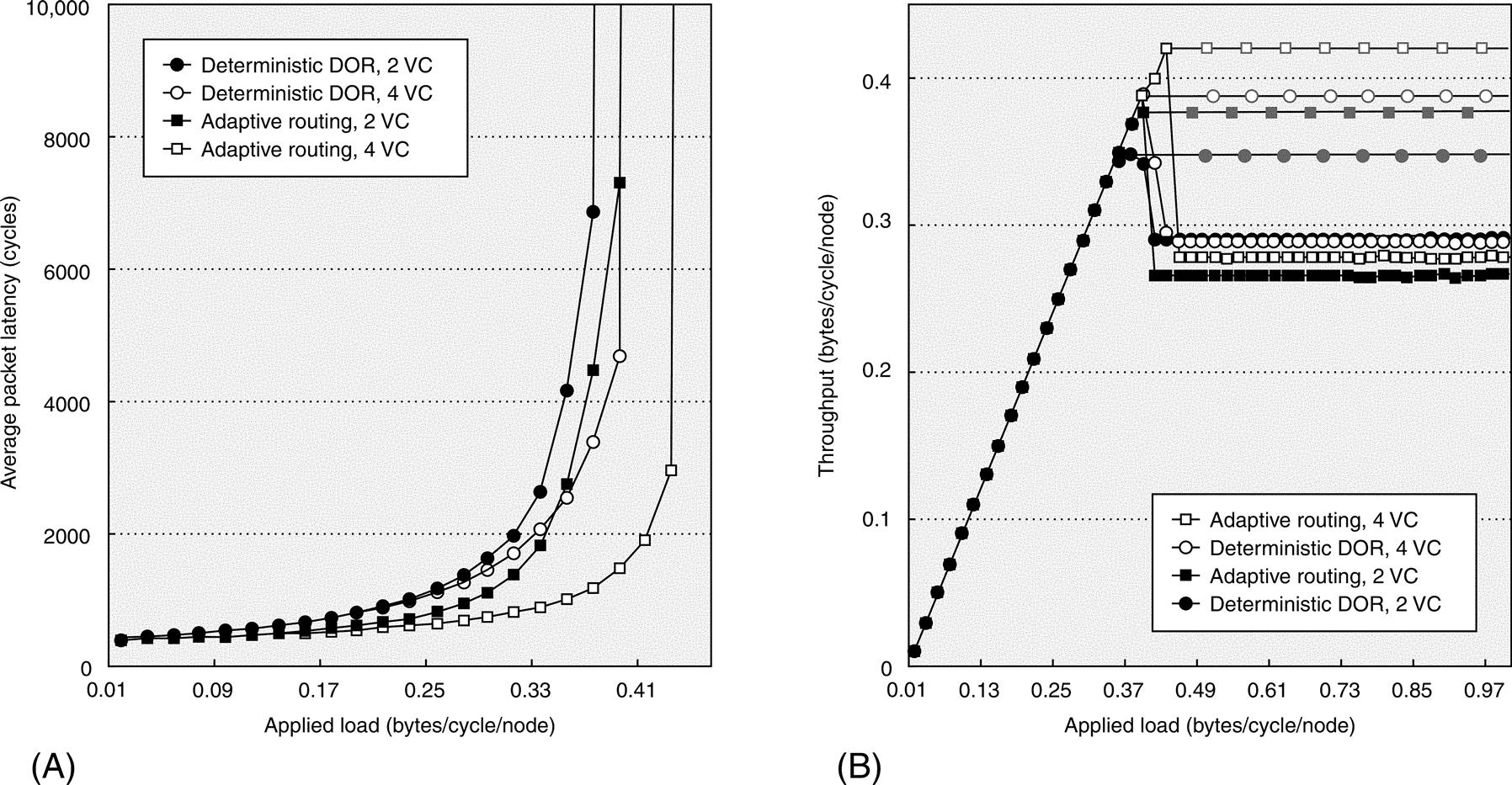
(a) Average latency is plotted versus applied load, and (b) throughput is plotted versus applied load (the upper grayish plots show peak throughput, and the lower black plots show sustained throughput). Simulation data were collected by P. Gilabert and J. Flich at the Universidad Politècnica de València, Spain (2006).
As can be seen, the plots within each graph have similar characteristic shapes, but they have different values. For the latency graph, all start at the no-load latency as predicted by the latency expression given above, then slightly increase with traffic load as contention for network resources increases. At higher applied loads, latency increases exponentially, and the network approaches its saturation point as it is unable to absorb the applied load, = causing packets to queue up at their source nodes awaiting injection. In these simulations, the queues keep growing over time, making latency tend toward infinity. However, in practice, queues reach their capacity and trigger the application to stall further packet generation, or the application throttles itself waiting for acknowledgments/responses to outstanding packets. Nevertheless, latency grows at a slower rate for adaptive routing as alternative paths are provided to packets along congested resources.
For this same reason, adaptive routing allows the network to reach a higher peak throughput for the same number of virtual channels as compared to deterministic routing. At nonsaturation loads, throughput increases fairly linearly with applied load. When the network reaches its saturation point, however, it is unable to deliver traffic at the same rate at which traffic is generated. The saturation point, therefore, indicates the maximum achievable or “peak” throughput, which would be no more than that predicted by the effective bandwidth expression given above. Beyond saturation, throughput tends to drop as a consequence of massive head-of-line blocking across the network (as will be explained further in Section F.6), very much like cars tend to advance more slowly at rush hour. This is an important region of the throughput graph as it shows how significant of a performance drop the routing algorithm can cause if congestion management techniques (discussed briefly in Section F.7) are not used effectively. In this case, adaptive routing has more of a performance drop after saturation than deterministic routing, as measured by the postsaturation sustained throughput.
For both routing algorithms, more virtual channels (i.e., four) give packets a greater ability to pass over blocked packets ahead, allowing for a higher peak throughput as compared to fewer virtual channels (i.e., two). For adaptive routing with four virtual channels, the peak throughput of 0.43 bytes/cycle/node is near the maximum of 0.5 bytes/cycle/node that can be obtained with 100% efficiency (i.e., ρ = 100%), assuming there is enough injection and reception bandwidth to make the network bisection the bottlenecking point. In that case, the network bandwidth is simply 100% times the network bisection bandwidth (BWBisection) divided by the fraction of traffic crossing the bisection (γ), as given by the expression above. Taking into account that the bisection splits the torus into two equally sized halves, γ is equal to 0.5 for uniform traffic as only half the injected traffic is destined to a node at the other side of the bisection. The BWBisection for a 4096-node 3D torus network is 16 × 16 × 4 unidirectional links times the link bandwidth (i.e., 1 byte/cycle). If we normalize the bisection bandwidth by dividing it by the number of nodes (as we did with network bandwidth), the BWBisection is 0.25 bytes/cycle/node. Dividing this by γ gives the ideal maximally obtainable network bandwidth of 0.5 bytes/cycle/node.
We can find the efficiency factor, ρ, of the simulated network simply by dividing the measured peak throughput by the ideal throughput. The efficiency factor for the network with fully adaptive routing and four virtual channels is 0.43/(0.25/0.5) = 86%, whereas for the network with deterministic routing and two virtual channels it is 0.37/(0.25/0.5) = 74%. Besides the 12% difference in efficiency between the two, another 14% gain in efficiency might be obtained with even better routing, arbitration, switching, and virtual channel designs.
To put this discussion on routing, arbitration, and switching in perspective, Figure F.20 lists the techniques used in SANs designed for commercial high-performance computers. In addition to being applied to the SANs as shown in the figure, the issues discussed in this section also apply to other interconnect domains: from OCNs to WANs.

F.6 Switch Microarchitecture
Network switches implement the routing, arbitration, and switching functions of switched-media networks. Switches also implement buffer management mechanisms and, in the case of lossless networks, the associated flow control. For some networks, switches also implement part of the network management functions that explore, configure, and reconfigure the network topology in response to boot-up and failures. Here, we reveal the internal structure of network switches by describing a basic switch microarchitecture and various alternatives suitable for different routing, arbitration, and switching techniques presented previously.
Basic Switch Microarchitecture
The internal data path of a switch provides connectivity among the input and output ports. Although a shared bus or a multiported central memory could be used, these solutions are insufficient or too expensive, respectively, when the required aggregate switch bandwidth is high. Most high-performance switches implement an internal crossbar to provide nonblocking connectivity within the switch, thus allowing concurrent connections between multiple input-output port pairs. Buffering of blocked packets can be done using first in, first out (FIFO) or circular queues, which can be implemented as dynamically allocatable multi-queues (DAMQs) in static RAM to provide high capacity and flexibility. These queues can be placed at input ports (i.e., input buffered switch), output ports (i.e., output buffered switch), centrally within the switch (i.e., centrally buffered switch), or at both the input and output ports of the switch (i.e., input-output-buffered switch). Figure F.21 shows a block diagram of an input-output-buffered switch.
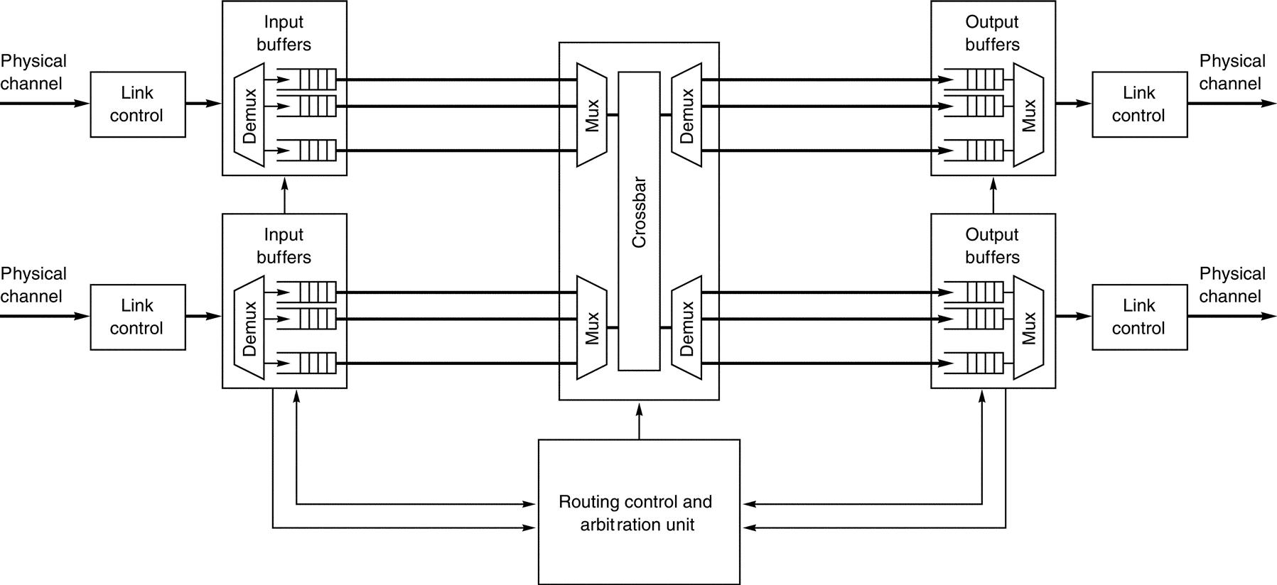
Routing can be implemented using a finite-state machine or forwarding table within the routing control unit of switches. In the former case, the routing information given in the packet header is processed by a finite-state machine that determines the allowed switch output port (or ports if routing is adaptive), according to the routing algorithm. Portions of the routing information in the header are usually stripped off or modified by the routing control unit after use to simplify processing at the next switch along the path. When routing is implemented using forwarding tables, the routing information given in the packet header is used as an address to access a forwarding table entry that contains the allowed switch output port(s) provided by the routing algorithm. Forwarding tables must be preloaded into the switches at the outset of network operation. Hybrid approaches also exist where the forwarding table is reduced to a small set of routing bits and combined with a small logic block. Those routing bits are used by the routing control unit to know what paths are allowed and decide the output ports the packets need to take. The goal with those approaches is to build flexible yet compact routing control units, eliminating the area and power wastage of a large forwarding table and thus being suitable for OCNs. The routing control unit is usually implemented as a centralized resource, although it could be replicated at every input port so as not to become a bottleneck. Routing is done only once for every packet, and packets typically are large enough to take several cycles to flow through the switch, so a centralized routing control unit rarely becomes a bottleneck. Figure F.21 assumes a centralized routing control unit within the switch.
Arbitration is required when two or more packets concurrently request the same output port, as described in the previous section. Switch arbitration can be implemented in a centralized or distributed way. In the former case, all of the requests and status information are transmitted to the central switch arbitration unit; in the latter case, the arbiter is distributed across the switch, usually among the input and/or output ports. Arbitration may be performed multiple times on packets, and there may be multiple queues associated with each input port, increasing the number of arbitration requests that must be processed. Thus, many implementations use a hierarchical arbitration approach, where arbitration is first performed locally at every input port to select just one request among the corresponding packets and queues, and later arbitration is performed globally to process the requests made by each of the local input port arbiters. Figure F.21 assumes a centralized arbitration unit within the switch.
The basic switch microarchitecture depicted in Figure F.21 functions in the following way. When a packet starts to arrive at a switch input port, the link controller decodes the incoming signal and generates a sequence of bits, possibly deserializing data to adapt them to the width of the internal data path if different from the external link width. Information is also extracted from the packet header or link control signals to determine the queue to which the packet should be buffered. As the packet is being received and buffered (or after the entire packet has been buffered, depending on the switching technique), the header is sent to the routing unit. This unit supplies a request for one or more output ports to the arbitration unit. Arbitration for the requested output port succeeds if the port is free and has enough space to buffer the entire packet or flit, depending on the switching technique. If wormhole switching with virtual channels is implemented, additional arbitration and allocation steps may be required for the transmission of each individual flit. Once the resources are allocated, the packet is transferred across the internal crossbar to the corresponding output buffer and link if no other packets are ahead of it and the link is free. Link-level flow control implemented by the link controller prevents input queue overflow at the neighboring switch on the other end of the link. If virtual channel switching is implemented, several packets may be time-multiplexed across the link on a flit-by-flit basis. As the various input and output ports operate independently, several incoming packets may be processed concurrently in the absence of contention.
Buffer Organizations
As mentioned above, queues can be located at the switch input, output, or both sides. Output-buffered switches have the advantage of completely eliminating head-of-line blocking. Head-of-line (HOL) blocking occurs when two or more packets are buffered in a queue, and a blocked packet at the head of the queue blocks other packets in the queue that would otherwise be able to advance if they were at the queue head. This cannot occur in output-buffered switches as all the packets in a given queue have the same status; they require the same output port. However, it may be the case that all the switch input ports simultaneously receive a packet for the same output port. As there are no buffers at the input side, output buffers must be able to store all those incoming packets at the same time. This requires implementing output queues with an internal switch speedup of k. That is, output queues must have a write bandwidth k times the link bandwidth, where k is the number of switch ports. This oftentimes is too expensive. Hence, this solution by itself has rarely been implemented in lossless networks. As the probability of concurrently receiving many packets for the same output port is usually small, commercial systems that use output-buffered switches typically implement only moderate switch speedup, dropping packets on rare buffer overflow.
Switches with buffers on the input side are able to receive packets without having any switch speedup; however, HOL blocking can occur within input port queues, as illustrated in Figure F.22(a). This can reduce switch output port utilization to less than 60% even when packet destinations are uniformly distributed. As shown in Figure F.22(b), the use of virtual channels (two in this case) can mitigate HOL blocking but does not eliminate it. A more effective solution is to organize the input queues as virtual output queues (VOQs), shown in Figure F.22(c). With this, each input port implements as many queues as there are output ports, thus providing separate buffers for packets destined to different output ports. This is a popular technique widely used in ATM switches and IP routers. The main drawbacks of VOQs, however, are cost and lack of scalability: The number of VOQs grows quadratically with switch ports. Moreover, although VOQs eliminate HOL blocking within a switch, HOL blocking occurring at the network level end-to-end is not solved. Of course, it is possible to design a switch with VOQ support at the network level also—that is, to implement as many queues per switch input port as there are output ports across the entire network—but this is extremely expensive. An alternative is to dynamically assign only a fraction of the queues to store (cache) separately only those packets headed for congested destinations.

The shaded input buffer is the one to which the crossbar is currently allocated. This assumes each input port has only one access port to the switch’s internal crossbar.
Combined input-output-buffered switches minimize HOL blocking when there is sufficient buffer space at the output side to buffer packets, and they minimize the switch speedup required due to buffers being at the input side. This solution has the further benefit of decoupling packet transmission through the internal crossbar of the switch from transmission through the external links. This is especially useful for cut-through switching implementations that use virtual channels, where flit transmissions are time-multiplexed over the links. Many designs used in commercial systems implement input-output-buffered switches.
Routing Algorithm Implementation
It is important to distinguish between the routing algorithm and its implementation. While the routing algorithm describes the rules to forward packets across the network and affects packet latency and network throughput, its implementation affects the delay suffered by packets when reaching a node, the required silicon area, and the power consumption associated with the routing computation. Several techniques have been proposed to pre-compute the routing algorithm and/or hide the routing computation delay. However, significantly less effort has been devoted to reduce silicon area and power consumption without significantly affecting routing flexibility. Both issues have become very important, particularly for OCNs. Many existing designs address these issues by implementing relatively simple routing algorithms, but more sophisticated routing algorithms will likely be needed in the future to deal with increasing manufacturing defects, process variability, and other complications arising from continued technology scaling, as discussed briefly below.
As mentioned in a previous section, depending on where the routing algorithm is computed, two basic forms of routing exist: source and distributed routing. In source routing, the complexity of implementation is moved to the end nodes where paths need to be stored in tables, and the path for a given packet is selected based on the destination end node identifier. In distributed routing, however, the complexity is moved to the switches where, at each hop along the path of a packet, a selection of the output port to take is performed. In distributed routing, two basic implementations exist. The first one consists of using a logic block that implements a fixed routing algorithm for a particular topology. The most common example of such an implementation is dimension-order routing, where dimensions are offset in an established order. Alternatively, distributed routing can be implemented with forwarding tables, where each entry encodes the output port to be used for a particular destination. Therefore, in the worst case, as many entries as destination nodes are required.
Both methods for implementing distributed routing have their benefits and drawbacks. Logic-based routing features a very short computation delay, usually requires a small silicon area, and has low power consumption. However, logicbased routing needs to be designed with a specific topology in mind and, therefore, is restricted to that topology. Table-based distributed routing is quite flexible and supports any topology and routing algorithm. Simply, tables need to be filled with the proper contents based on the applied routing algorithm (e.g., the up*/down* routing algorithm can be defined for any irregular topology). However, the down side of table-based distributed routing is its non-negligible area and power cost. Also, scalability is problematic in table-based solutions as, in the worst case, a system with N end nodes (and switches) requires as many as N tables each with N entries, thus having quadratic cost.
Depending on the network domain, one solution is more suitable than the other. For instance, in SANs, it is usual to find table-based solutions as is the case with InfiniBand. In other environments, like OCNs, table-based implementations are avoided due to the aforementioned costs in power and silicon area. In such environments, it is more advisable to rely on logic-based implementations. Herein lies some of the challenges OCN designers face: ever continuing technology scaling through device miniaturization leads to increases in the number of manufacturing defects, higher failure rates (either transient or permanent), significant process variations (transistors behaving differently from design specs), the need for different clock frequency and voltage domains, and tight power and energy budgets. All of these challenges translate to the network needing support for heterogeneity. Different—possibly irregular—regions of the network will be created owing to failed components, powered down switches and links, disabled components (due to unacceptable variations in performance) and so on. Hence, heterogeneous systems may emerge from a homogeneous design. In this framework, it is important to efficiently implement routing algorithms designed to provide enough flexibility to address these new challenges.
A well-known solution for providing a certain degree of flexibility while being much more compact than traditional table-based approaches is interval routing [Leeuwen 1987], where a range of destinations is defined for each output port. Although this approach is not flexible enough, it provides a clue on how to address emerging challenges. A more recent approach provides a plausible implementation design point that lies between logic-based implementation (efficiency) and table-based implementation (flexibility). Logic-Based Distributed Routing (LBDR) is a hybrid approach that takes as a reference a regular 2D mesh but allows an irregular network to be derived from it due to changes in topology induced by manufacturing defects, failures, and other anomalies. Due to the faulty, disabled, and powered-down components, regularity is compromised and the dimension-order routing algorithm can no longer be used. To support such topologies, LBDR defines a set of configuration bits at each switch. Four connectivity bits are used at each switch to indicate the connectivity of the switch to the neighbor switches in the topology. Thus, one connectivity bit per port is used. Those connectivity bits are used, for instance, to disable an output port leading to a faulty component. Additionally, eight routing bits are used, two per output port, to define the available routing options. The value of the routing bits is set at power-on and is computed from the routing algorithm to be implemented in the network. Basically, when a routing bit is set, it indicates that a packet can leave the switch through the associated output port and is allowed to perform a certain turn at the next switch. In this respect, LBDR is similar to interval routing, but it defines geographical areas instead of ranges of destinations. Figure F.23 shows an example where a topology-agnostic routing algorithm is implemented with LBDR on an irregular topology. The figure shows the computed configuration bits.

For each router, connectivity and routing bits are defined.
The connectivity and routing bits are used to implement the routing algorithm. For that purpose, a small set of logic gates are used in combination with the configuration bits. Basically, the LBDR approach takes as a reference the initial topology (a 2D mesh), and makes a decision based on the current coordinates of the router, the coordinates of the destination router, and the configuration bits. Figure F.24 shows the required logic, and Figure F.25 shows an example of where a packet is forwarded from its source to its destination with the use of the configuration bits. As can be noticed, routing restrictions are enforced by preventing the use of the west port at switch 10.


LBDR represents a method for efficient routing implementation in OCNs. This mechanism has been recently extended to support non-minimal paths, collective communication operations, and traffic isolation. All of these improvements have been made while maintaining a compact and efficient implementation with the use of a small set of configuration bits. A detailed description of LBDR and its extensions, and the current research on OCNs can be found in Flich [2010].
Pipelining the Switch Microarchitecture
Performance can be enhanced by pipelining the switch microarchitecture. Pipelined processing of packets in a switch has similarities with pipelined execution of instructions in a vector processor. In a vector pipeline, a single instruction indicates what operation to apply to all the vector elements executed in a pipelined way. Similarly, in a switch pipeline, a single packet header indicates how to process all of the internal data path physical transfer units (or phits) of a packet, which are processed in a pipelined fashion. Also, as packets at different input ports are independent of each other, they can be processed in parallel similar to the way multiple independent instructions or threads of pipelined instructions can be executed in parallel.
The switch microarchitecture can be pipelined by analyzing the basic functions performed within the switch and organizing them into several stages. Figure F.26 shows a block diagram of a five-stage pipelined organization for the basic switch microarchitecture given in Figure F.21, assuming cut-through switching and the use of a forwarding table to implement routing. After receiving the header portion of the packet in the first stage, the routing information (i.e., destination address) is used in the second stage to look up the allowed routing option(s) in the forwarding table. Concurrent with this, other portions of the packet are received and buffered in the input port queue at the first stage. Arbitration is performed in the third stage. The crossbar is configured to allocate the granted output port for the packet in the fourth stage, and the packet header is buffered in the switch output port and ready for transmission over the external link in the fifth stage. Note that the second and third stages are used only by the packet header; the payload and trailer portions of the packet use only three of the stages—those used for data flow-thru once the internal data path of the switch is set up.
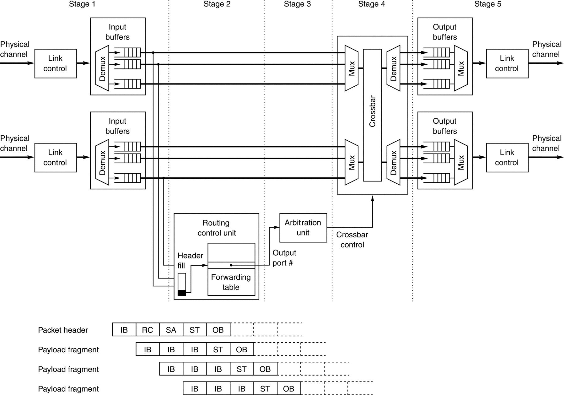
The notation in the figure is as follows: IB is the input link control and buffer stage, RC is the route computation stage, SA is the crossbar switch arbitration stage, ST is the crossbar switch traversal stage, and OB is the output buffer and link control stage. Packet fragments (flits) coming after the header remain in the IB stage until the header is processed and the crossbar switch resources are provided.
A virtual channel switch usually requires an additional stage for virtual channel allocation. Moreover, arbitration is required for every flit before transmission through the crossbar. Finally, depending on the complexity of the routing and arbitration algorithms, several clock cycles may be required for these operations.
Other Switch Microarchitecture Enhancements
As mentioned earlier, internal switch speedup is sometimes implemented to increase switch output port utilization. This speedup is usually implemented by increasing the clock frequency and/or the internal data path width (i.e., phit size) of the switch. An alternative solution consists of implementing several parallel data paths from each input port’s set of queues to the output ports. One way of doing this is by increasing the number of crossbar input ports. When implementing several physical queues per input port, this can be achieved by devoting a separate crossbar port to each input queue. For example, the IBM Blue Gene/L implements two crossbar access ports and two read ports per switch input port.
Another way of implementing parallel data paths between input and output ports is to move the buffers to the crossbar crosspoints. This switch architecture is usually referred to as a buffered crossbar switch. A buffered crossbar provides independent data paths from each input port to the different output ports, thus making it possible to send up to k packets at a time from a given input port to k different output ports. By implementing independent crosspoint memories for each input-output port pair, HOL blocking is eliminated at the switch level. Moreover, arbitration is significantly simpler than in other switch architectures. Effectively, each output port can receive packets from only a disjoint subset of the crosspoint memories. Thus, a completely independent arbiter can be implemented at each switch output port, each of those arbiters being very simple.
A buffered crossbar would be the ideal switch architecture if it were not so expensive. The number of crosspoint memories increases quadratically with the number of switch ports, dramatically increasing its cost and reducing its scalability with respect to the basic switch architecture. In addition, each crosspoint memory must be large enough to efficiently implement link-level flow control. To reduce cost, most designers prefer input-buffered or combined input-output-buffered switches enhanced with some of the mechanisms described previously.
F.7 Practical Issues for Commercial Interconnection Networks
There are practical issues in addition to the technical issues described thus far that are important considerations for interconnection networks within certain domains. We mention a few of these below.
Connectivity
The type and number of devices that communicate and their communication requirements affect the complexity of the interconnection network and its protocols. The protocols must target the largest network size and handle the types of anomalous systemwide events that might occur. Among some of the issues are the following: How lightweight should the network interface hardware/software be? Should it attach to the memory network or the I/O network? Should it support cache coherence? If the operating system must get involved for every network transaction, the sending and receiving overhead becomes quite large. If the network interface attaches to the I/O network (PCI-Express or HyperTransport interconnect), the injection and reception bandwidth will be limited to that of the I/O network. This is the case for the Cray XT3 SeaStar, Intel Thunder Tiger 4 QsNetII, and many other supercomputer and cluster networks. To support coherence, the sender may have to flush the cache before each send, and the receiver may have to flush its cache before each receive to prevent the stale-data problem. Such flushes further increase sending and receiving overhead, often causing the network interface to be the network bottleneck.
Computer systems typically have a multiplicity of interconnects with different functions and cost-performance objectives. For example, processor-memory interconnects usually provide higher bandwidth and lower latency than I/O interconnects and are more likely to support cache coherence, but they are less likely to follow or become standards. Personal computers typically have a processormemory interconnect and an I/O interconnect (e.g., PCI-X 2.0, PCIe or Hyper-Transport) designed to connect both fast and slow devices (e.g., USB 2.0, Gigabit Ethernet LAN, Firewire 800). The Blue Gene/L supercomputer uses five interconnection networks, only one of which is the 3D torus used for most of the interprocessor application traffic. The others include a tree-based collective communication network for broadcast and multicast; a tree-based barrier network for combining results (scatter, gather); a control network for diagnostics, debugging, and initialization; and a Gigabit Ethernet network for I/O between the nodes and disk. The University of Texas at Austin’s TRIPS Edge processor has eight specialized on-chip networks—some with bidirectional channels as wide as 128 bits and some with 168 bits in each direction—to interconnect the 106 heterogeneous tiles composing the two processor cores with L2 on-chip cache. It also has a chip-to-chip switched network to interconnect multiple chips in a multiprocessor configuration. Two of the on-chip networks are switched networks: One is used for operand transport and the other is used for on-chip memory communication. The others are essentially fan-out trees or recombination dedicated link networks used for status and control. The portion of chip area allocated to the interconnect is substantial, with five of the seven metal layers used for global network wiring.
Standardization: Cross-Company Interoperability
Standards are useful in many places in computer design, including interconnection networks. Advantages of successful standards include low cost and stability. The customer has many vendors to choose from, which keeps price close to cost due to competition. It makes the viability of the interconnection independent of the stability of a single company. Components designed for a standard interconnection may also have a larger market, and this higher volume can reduce the vendors’ costs, further benefiting the customer. Finally, a standard allows many companies to build products with interfaces to the standard, so the customer does not have to wait for a single company to develop interfaces to all the products of interest.
One drawback of standards is the time it takes for committees and special-interest groups to agree on the definition of standards, which is a problem when technology is changing rapidly. Another problem is when to standardize: On the one hand, designers would like to have a standard before anything is built; on the other hand, it would be better if something were built before standardization to avoid legislating useless features or omitting important ones. When done too early, it is often done entirely by committee, which is like asking all of the chefs in France to prepare a single dish of food—masterpieces are rarely served. Standards can also suppress innovation at that level, since standards fix the interfaces—at least until the next version of the standards surface, which can be every few years or longer. More often, we are seeing consortiums of companies getting together to define and agree on technology that serve as “de facto” industry standards. This was the case for InfiniBand.
LANs and WANs use standards and interoperate effectively. WANs involve many types of companies and must connect to many brands of computers, so it is difficult to imagine a proprietary WAN ever being successful. The ubiquitous nature of the Ethernet shows the popularity of standards for LANs as well as WANs, and it seems unlikely that many customers would tie the viability of their LAN to the stability of a single company. Some SANs are standardized such as Fibre Channel, but most are proprietary. OCNs for the most part are proprietary designs, with a few gaining widespread commercial use in system-on-chip (SoC) applications, such as IBM’s CoreConnect and ARM’s AMBA.
Congestion Management
Congestion arises when too many packets try to use the same link or set of links. This leads to a situation in which the bandwidth required exceeds the bandwidth supplied. Congestion by itself does not degrade network performance: simply, the congested links are running at their maximum capacity. Performance degradation occurs in the presence of HOL blocking where, as a consequence of packets going to noncongested destinations getting blocked by packets going to congested destinations, some link bandwidth is wasted and network throughput drops, as illustrated in the example given at the end of Section F.4. Congestion control refers to schemes that reduce traffic when the collective traffic of all nodes is too large for the network to handle.
One advantage of a circuit-switched network is that, once a circuit is established, it ensures that there is sufficient bandwidth to deliver all the information sent along that circuit. Interconnection bandwidth is reserved as circuits are established, and if the network is full, no more circuits can be established. Other switching techniques generally do not reserve interconnect bandwidth in advance, so the interconnection network can become clogged with too many packets. Just as with poor rush-hour commuters, a traffic jam of packets increases packet latency and, in extreme cases, fewer packets per second get delivered by the interconnect. In order to handle congestion in packet-switched networks, some form of congestion management must be implemented. The two kinds of mechanisms used are those that control congestion and those that eliminate the performance degradation introduced by congestion.
There are three basic schemes used for congestion control in interconnection networks, each with its own weaknesses: packet discarding, flow control, and choke packets. The simplest scheme is packet discarding, which we discussed briefly in Section F.2. If a packet arrives at a switch and there is no room in the buffer, the packet is discarded. This scheme relies on higher-level software that handles errors in transmission to resend lost packets. This leads to significant bandwidth wastage due to (re)transmitted packets that are later discarded and, therefore, is typically used only in lossy networks like the Internet.
The second scheme relies on flow control, also discussed previously. When buffers become full, link-level flow control provides feedback that prevents the transmission of additional packets. This backpressure feedback rapidly propagates backward until it reaches the sender(s) of the packets producing congestion, forcing a reduction in the injection rate of packets into the network. The main drawbacks of this scheme are that sources become aware of congestion too late when the network is already congested, and nothing is done to alleviate congestion. Backpressure flow control is common in lossless networks like SANs used in supercomputers and enterprise systems.
A more elaborate way of using flow control is by implementing it directly between the sender and the receiver end nodes, generically called end-to-end flow control. Windowing is one version of end-to-end credit-based flow control where the window size should be large enough to efficiently pipeline packets through the network. The goal of the window is to limit the number of unacknowledged packets, thus bounding the contribution of each source to congestion, should it arise. The TCP protocol uses a sliding window. Note that end-to-end flow control describes the interaction between just two nodes of the interconnection network, not the entire interconnection network between all end nodes. Hence, flow control helps congestion control, but it is not a global solution.
Choke packets are used in the third scheme, which is built upon the premise that traffic injection should be throttled only when congestion exists across the network. The idea is for each switch to see how busy it is and to enter into a warning state when it passes a threshold. Each packet received by a switch in the warning state is sent back to the source via a choke packet that includes the intended destination. The source is expected to reduce traffic to that destination by a fixed percentage. Since it likely will have already sent other packets along that path, the source node waits for all the packets in transit to be returned before acting on the choke packets. In this scheme, congestion is controlled by reducing the packet injection rate until traffic reduces, just as metering lights that guard on-ramps control the rate of cars entering a freeway. This scheme works efficiently when the feedback delay is short. When congestion notification takes a long time, usually due to long time of flight, this congestion control scheme may become unstable—reacting too slowly or producing oscillations in packet injection rate, both of which lead to poor network bandwidth utilization.
An alternative to congestion control consists of eliminating the negative consequences of congestion. This can be done by eliminating HOL blocking at every switch in the network as discussed previously. Virtual output queues can be used for this purpose; however, it would be necessary to implement as many queues at every switch input port as devices attached to the network. This solution is very expensive, and not scalable at all. Fortunately, it is possible to achieve good results by dynamically assigning a few set-aside queues to store only the congested packets that travel through some hot-spot regions of the network, very much like caches are intended to store only the more frequently accessed memory locations. This strategy is referred to as regional explicit congestion notification (RECN).
Fault Tolerance
The probability of system failures increases as transistor integration density and the number of devices in the system increases. Consequently, system reliability and availability have become major concerns and will be even more important in future systems with the proliferation of interconnected devices. A practical issue arises, therefore, as to whether or not the interconnection network relies on all the devices being operational in order for the network to work properly. Since software failures are generally much more frequent than hardware failures, another question surfaces as to whether a software crash on a single device can prevent the rest of the devices from communicating. Although some hardware designers try to build fault-free networks, in practice, it is only a question of the rate of failures, not whether they can be prevented. Thus, the communication subsystem must have mechanisms for dealing with faults when—not if—they occur.
There are two main kinds of failure in an interconnection network: transient and permanent. Transient failures are usually produced by electromagnetic interference and can be detected and corrected using the techniques described in Section F.2. Oftentimes, these can be dealt with simply by retransmitting the packet either at the link level or end-to-end. Permanent failures occur when some component stops working within specifications. Typically, these are produced by overheating, overbiasing, overuse, aging, and so on and cannot be recovered from simply by retransmitting packets with the help of some higher-layer software protocol. Either an alternative physical path must exist in the network and be supplied by the routing algorithm to circumvent the fault or the network will be crippled, unable to deliver packets whose only paths are through faulty resources.
Three major categories of techniques are used to deal with permanent failures: resource sparing, fault-tolerant routing, and network reconfiguration. In the first technique, faulty resources are switched off or bypassed, and some spare resources are switched in to replace the faulty ones. As an example, the ServerNet interconnection network is designed with two identical switch fabrics, only one of which is usable at any given time. In case of failure in one fabric, the other is used. This technique can also be implemented without switching in spare resources, leading to a degraded mode of operation after a failure. The IBM Blue Gene/L supercomputer, for instance, has the facility to bypass failed network resources while retaining its base topological structure and routing algorithm. The main drawback of this technique is the relatively large number of healthy resources (e.g., midplane node boards) that may need to be switched off after a failure in order to retain the base topological structure (e.g., a 3D torus).
Fault-tolerant routing, on the other hand, takes advantage of the multiple paths already existing in the network topology to route messages in the presence of failures without requiring spare resources. Alternative paths for each supported fault combination are identified at design time and incorporated into the routing algorithm. When a fault is detected, a suitable alternative path is used. The main difficulty when using this technique is guaranteeing that the routing algorithm will remain deadlock-free when using the alternative paths, given that arbitrary fault patterns may occur. This is especially difficult in direct networks whose regularity can be compromised by the fault pattern. The Cray T3E is an example system that successfully applies this technique on its 3D torus direct network. There are many examples of this technique in systems using indirect networks, such as with the bidirectional multistage networks in the ASCI White and ASC Purple. Those networks provide multiple minimal paths between end nodes and, inherently, have no routing deadlock problems (see Section F.5). In these networks, alternative paths are selected at the source node in case of failure.
Network reconfiguration is yet another, more general technique to handle voluntary and involuntary changes in the network topology due either to failures or to some other cause. In order for the network to be reconfigured, the nonfaulty portions of the topology must first be discovered, followed by computation of the new routing tables and distribution of the routing tables to the corresponding network locations (i.e., switches and/or end node devices). Network reconfiguration requires the use of programmable switches and/or network interfaces, depending on how routing is performed. It may also make use of generic routing algorithms (e.g., up*/down* routing) that can be configured for all the possible network topologies that may result after faults. This strategy relieves the designer from having to supply alternative paths for each possible fault combination at design time. Programmable network components provide a high degree of flexibility but at the expense of higher cost and latency. Most standard and proprietary interconnection networks for clusters and SANs—including Myrinet, Quadrics, InfiniBand, Advanced Switching, and Fibre Channel—incorporate software for (re)configuring the network routing in accordance with the prevailing topology.
Another practical issue ties to node failure tolerance. If an interconnection network can survive a failure, can it also continue operation while a new node is added to or removed from the network, usually referred to as hot swapping? If not, each addition or removal of a new node disables the interconnection network, which is impractical for WANs and LANs and is usually intolerable for most SANs. Online system expansion requires hot swapping, so most networks allow for it. Hot swapping is usually supported by implementing dynamic network reconfiguration, in which the network is reconfigured without having to stop user traffic. The main difficulty with this is guaranteeing deadlock-free routing while routing tables for switches and/or end node devices are dynamically and asynchronously updated as more than one routing algorithm may be alive (and, perhaps, clashing) in the network at the same time. Most WANs solve this problem by dropping packets whenever required, but dynamic network reconfiguration is much more complex in lossless networks. Several theories and practical techniques have recently been developed to address this problem efficiently.
Example
Figure F.27 shows the number of failures of 58 desktop computers on a local area network for a period of just over one year. Suppose that one local area network is based on a network that requires all machines to be operational for the interconnection network to send data; if a node crashes, it cannot accept messages, so the interconnection becomes choked with data waiting to be delivered. An alternative is the traditional local area network, which can operate in the presence of node failures; the interconnection simply discards messages for a node that decides not to accept them. Assuming that you need to have both your workstation and the connecting LAN to get your work done, how much greater are your chances of being prevented from getting your work done using the failure-intolerant LAN versus traditional LANs? Assume the downtime for a crash is less than 30 minutes. Calculate using the one-hour intervals from this figure.

These reboots are distributed into time intervals of one hour and one day. The first column sorts the intervals according to the number of machines that failed in that interval. The next two columns concern one-hour intervals, and the last two columns concern one-day intervals. The second and fourth columns show the number of intervals for each number of failed machines. The third and fifth columns are just the product of the number of failed machines and the number of intervals. For example, there were 50 occurrences of one-hour intervals with 2 failed machines, for a total of 100 failed machines, and there were 35 days with 2 failed machines, for a total of 70 failures. As we would expect, the number of failures per interval changes with the size of the interval. For example, the day with 31 failures might include one hour with 11 failures and one hour with 20 failures. The last row shows the total number of each column; the number of failures doesn’t agree because multiple reboots of the same machine in the same interval do not result in separate entries. (Randy Wang of the University of California–Berkeley collected these data.)
Answer
Assuming the numbers for Figure F.27, the percentage of hours that you can’t get your work done using the failure-intolerant network is

The percentage of hours that you can’t get your work done using the traditional network is just the time your workstation has crashed. If these failures are equally distributed among workstations, the percentage is

Hence, you are more than 30 times more likely to be prevented from getting your work done with the failure-intolerant LAN than with the traditional LAN, according to the failure statistics in Figure F.27. Stated alternatively, the person responsible for maintaining the LAN would receive a 30-fold increase in phone calls from irate users!
F.8 Examples of Interconnection Networks
To further provide mass to the concepts described in the previous sections, we look at five example networks from the four interconnection network domains considered in this appendix. In addition to one for each of the OCN, LAN, and WAN areas, we look at two examples from the SAN area: one for system area networks and one for system/storage area networks. The first two examples are proprietary networks used in high-performance systems; the latter three examples are network standards widely used in commercial systems.
On-Chip Network: Intel Single-Chip Cloud Computer
With continued increases in transistor integration as predicted by Moore’s law, processor designers are under the gun to find ways of combating chip-crossing wire delay and other problems associated with deep submicron technology scaling. Multicore microarchitectures have gained popularity, given their advantages of simplicity, modularity, and ability to exploit parallelism beyond that which can be achieved through aggressive pipelining and multiple instruction/data issuing on a single core. No matter whether the processor consists of a single core or multiple cores, higher and higher demands are being placed on intrachip communication bandwidth to keep pace—not to mention interchip bandwidth. This has spurred a great amount of interest in OCN designs that efficiently support communication of instructions, register operands, memory, and I/O data within and between processor cores both on and off the chip. Here we focus on one such on-chip network: The Intel Single-chip Cloud Computer prototype.
The Single-chip Cloud Computer (SCC) is a prototype chip multiprocessor with 48 Intel IA-32 architecture cores. Cores are laid out (see Figure F.28) on a network with a 2D mesh topology (6 × 4). The network connects 24 tiles, 4 on-die memory controllers, a voltage regulator controller (VRC), and an external system interface controller (SIF). In each tile two cores are connected to a router. The four memory controllers are connected at the boundaries of the mesh, two on each side, while the VRC and SIF controllers are connected at the bottom border of the mesh.

Each memory controller can address two DDR3 DIMMS, each up to 8 GB of memory, thus resulting in a maximum of 64 GB of memory. The VRC controller allows any core or the system interface to adjust the voltage in any of the six pre-defined regions configuring the network (two 2-tile regions). The clock can also be adjusted at a finer granularity with each tile having its own operating frequency. These regions can be turned off or scaled down for large power savings. This method allows full application control of the power state of the cores. Indeed, applications have an API available to define the voltage and the frequency of each region. The SIF controller is used to communicate the network from outside the chip.
Each of the tiles includes two processor cores (P54C-based IA) with associated L1 16 KB data cache and 16 KB instruction cache and a 256 KB L2 cache (with the associated controller), a 5-port router, traffic generator (for testing purposes only), a mesh interface unit (MIU) handling all message passing requests, memory look-up tables (with configuration registers to set the mapping of a core’s physical addresses to the extended memory map of the system), a message-passing buffer, and circuitry for the clock generation and synchronization for crossing asynchronous boundaries.
Focusing on the OCN, the MIU unit is in charge of interfacing the cores to the network, including the packetization and de-packetization of large messages; command translation and address decoding/lookup; link-level flow control and credit management; and arbiter decisions following a round-robin scheme. A credit-based flow control mechanism is used together with virtual cut-through switching (thus making it necessary to split long messages into packets). The routers are connected in a 2D mesh layout, each on its own power supply and clock source. Links connecting routers have 16B + 2B side bands running at 2 GHz. Zero-load latency is set to 4 cycles, including link traversal. Eight virtual channels are used for performance (6 VCs) and protocol-level deadlock handling (2 VCs). A message-level arbitration is implemented by a wrapped wave-front arbiter. The dimension-order XY routing algorithm is used and pre-computation of the output port is performed at every router.
Besides the tiles having regions defined for voltage and frequency, the network (made of routers and links) has its own single region. Thus, all the network components run at the same speed and use the same power supply. An asynchronous clock transition is required between the router and the tile.
One of the distinctive features of the SCC architecture is the support for a messaging-based communication protocol rather than hardware cache-coherent memory for inter-core communication. Message passing buffers are located on every router and APIs are provided to take full control of MPI structures. Cache coherency can be implemented by software.
The SCC router represents a significant improvement over the Teraflops processor chip in the implementation of a 2D on-chip interconnect. Contrasted with the 2D mesh implemented in the Teraflops processor, this implementation is tuned for a wider data path in a multiprocessor interconnect and is more latency, area, and power optimized for such a width. It targets a lower 2-GHz frequency of operation compared to the 5 GHz of its predecessor Teraflops processor, yet with a higher-performance interconnect architecture.
System Area Network: IBM Blue Gene/L 3D Torus Network
The IBM BlueGene/L was the largest-scaled, highest-performing computer system in the world in 2005, according to www.top500.org. With 65,536 dual-processor compute nodes and 1024 I/O nodes, this 360 TFLOPS (peak) supercomputer has a system footprint of approximately 2500 square feet. Both processors at each node can be used for computation and can handle their own communication protocol processing in virtual mode or, alternatively, one of the processors can be used for computation and the other for network interface processing. Packets range in size from 32 bytes to a maximum of 256 bytes, and 8 bytes are used for the header. The header includes routing, virtual channel, link-level flow control, packet size, and other such information, along with 1 byte for CRC to protect the header. Three bytes are used for CRC at the packet level, and 1 byte serves as a valid indicator.
The main interconnection network is a proprietary 32 × 32 × 64 3D torus SAN that interconnects all 64 K nodes. Each node switch has six 350 MB/sec bidirectional links to neighboring torus nodes, an injection bandwidth of 612.5 MB/sec from the two node processors, and a reception bandwidth of 1050 MB/sec to the two node processors. The reception bandwidth from the network equals the inbound bandwidth across all switch ports, which prevents reception links from bottlenecking network performance. Multiple packets can be sunk concurrently at each destination node because of the higher reception link bandwidth.
Two nodes are implemented on a 2 × 1 × 1 compute card, 16 compute cards and 2 I/O cards are implemented on a 4 × 4 × 2 node board, 16 node boards are implemented on an 8 × 8 × 8 midplane, and 2 midplanes form a 1024-node rack with physical dimensions of 0.9 × 0.9 × 1.9 cubic meters. Links have a maximum physical length of 8.6 meters, thus enabling efficient link-level flow control with reasonably low buffering requirements. Low latency is achieved by implementing virtual cut-through switching, distributing arbitration at switch input and output ports, and precomputing the current routing path at the previous switch using a finite-state machine so that part of the routing delay is removed from the critical path in switches. High effective bandwidth is achieved using input-buffered switches with dual read ports, virtual cut-through switching with four virtual channels, and fully adaptive deadlock-free routing based on bubble flow control.
A key feature in networks of this size is fault tolerance. Failure rate is reduced by using a relatively low link clock frequency of 700 MHz (same as processor clock) on which both edges of the clock are used (i.e., 1.4 Gbps or 175 MB/sec transfer rate is supported for each bit-serial network link in each direction), but failures may still occur in the network. In case of failure, the midplane node boards containing the fault(s) are switched off and bypassed to isolate the fault, and computation resumes from the last checkpoint. Bypassing is done using separate bypass switch boards associated with each midplane that are additional to the set of torus node boards. Each bypass switch board can be configured to connect either to the corresponding links in the midplane node boards or to the next bypass board, effectively removing the corresponding set of midplane node boards. Although the number of processing nodes is reduced to some degree in some network dimensions, the machine retains its topological structure and routing algorithm.
Some collective communication operations such as barrier synchronization, broadcast/multicast, reduction, and so on are not performed well on the 3D torus as the network would be flooded with traffic. To remedy this, two separate tree networks with higher per-link bandwidth are used to implement collective and combining operations more efficiently. In addition to providing support for efficient synchronization and broadcast/multicast, hardware is used to perform some arithmetic reduction operations in an efficient way (e.g., to compute the sum or the maximum value of a set of values, one from each processing node). In addition to the 3D torus and the two tree networks, the Blue Gene/L implements an I/O Gigabit Ethernet network and a control system Fast Ethernet network of lower bandwidth to provide for parallel I/O, configuration, debugging, and maintenance.
System/Storage Area Network: InfiniBand
InfiniBand is an industrywide de facto networking standard developed in October 2000 by a consortium of companies belonging to the InfiniBand Trade Association. InfiniBand can be used as a system area network for interprocessor communication or as a storage area network for server I/O. It is a switch-based interconnect technology that provides flexibility in the topology, routing algorithm, and arbitration technique implemented by vendors and users. InfiniBand supports data transmission rates of 2 to 120 Gbp/link per direction across distances of 300 meters. It uses cut-through switching, 16 virtual channels and service levels, credit-based link-level flow control, and weighted round-robin fair scheduling and implements programmable forwarding tables. It also includes features useful for increasing reliability and system availability, such as communication subnet management, end-to-end path establishment, and virtual destination naming. Figure F.30 shows the packet format for InfiniBand juxtaposed with two other network standards from the LAN and WAN areas. Figure F.31 compares various characteristics of the InfiniBand standard with two proprietary system area networks widely used in research and commercial high-performance computer systems.

Some processors implement multiple on-chip networks (not all shown)—for example, two in the MIT Raw and eight in the TRIP Edge.

ATM calls their messages “cells” instead of packets, so the proper name is ATM cell format. The width of each drawing is 32 bits. All three formats have destination addressing fields, encoded differently for each situation. All three also have a checksum field to catch transmission errors, although the ATM checksum field is calculated only over the header; ATM relies on higher-level protocols to catch errors in the data. Both InfiniBand and Ethernet have a length field, since the packets hold a variable amount of data, with the former counted in 32-bit words and the latter in bytes. InfiniBand and ATM headers have a type field (T) that gives the type of packet. The remaining Ethernet fields are a preamble to allow the receiver to recover the clock from the self-clocking code used on the Ethernet, the source address, and a pad field to make sure the smallest packet is 64 bytes (including the header). InfiniBand includes a version field for protocol version, a sequence number to allow in-order delivery, a field to select the destination queue, and a partition key field. Infiniband has many more small fields not shown and many other packet formats; above is a simplified view. ATM’s short, fixed packet is a good match to real-time demand of digital voice.

InfiniBand offers two basic mechanisms to support user-level communication: send/receive and remote DMA (RDMA). With send/receive, the receiver has to explicitly post a receive buffer (i.e., allocate space in its channel adapter network interface) before the sender can transmit data. With RDMA, the sender can remotely DMA data directly into the receiver device’s memory. For example, for a nominal packet size of 4 bytes measured on a Mellanox MHEA28-XT channel adapter connected to a 3.4 GHz Intel Xeon host device, sending and receiving overhead is 0.946 and 1.423 μs, respectively, for the send/receive mechanism, whereas it is 0.910 and 0.323 μs, respectively, for the RDMA mechanism.
As discussed in Section F.2, the packet size is important in getting full benefit of the network bandwidth. One might ask, “What is the natural size of messages?” Figure F.32(a) shows the size of messages for a commercial fluid dynamics simulation application, called Fluent, collected on an InfiniBand network at The Ohio State University’s Network-Based Computer Laboratory. One plot is cumulative in messages sent and the other is cumulative in data bytes sent. Messages in this graph are message passing interface (MPI) units of information, which gets divided into InfiniBand maximum transfer units (packets) transferred over the network. As shown, the maximum message size is over 512 KB, but approximately 90% of the messages are less than 512 bytes. Messages of 2 KB represent approximately 50% of the bytes transferred. An Integer Sort application kernel in the NAS Parallel Benchmark suite is also measured to have about 75% of its messages below 512 bytes (plots not shown). Many applications send far more small messages than large ones, particularly since requests and acknowledgments are more frequent than data responses and block writes.

(a) Cumulative percentage of messages and volume of data transferred as message size varies for the Fluent application (www.fluent.com). Each x-axis entry includes all bytes up to the next one; for example, 128 represents 1 byte to 128 bytes. About 90% of the messages are less than 512 bytes, which represents about 40% of the total bytes transferred. (b) Effective bandwidth versus message size measured on SDR and DDR InfiniBand networks running MVAPICH (http://nowlab.cse.ohio-state.edu/projects/mpi-iba) with OS bypass (native) and without (IPoIB).
InfiniBand reduces protocol processing overhead by allowing it to be offloaded from the host computer to a controller on the InfiniBand network interface card. The benefits of protocol offloading and bypassing the operating system are shown in Figure F.32(b) for MVAPICH, a widely used implementation of MPI over InfiniBand. Effective bandwidth is plotted against message size for MVAPICH configured in two modes and two network speeds. One mode runs IPoIB, in which InfiniBand communication is handled by the IP layer implemented by the host’s operating system (i.e., no OS bypass). The other mode runs MVAPICH directly over VAPI, which is the native Mellanox InfiniBand interface that offloads transport protocol processing to the channel adapter hardware (i.e., OS bypass). Results are shown for 10 Gbps single data rate (SDR) and 20 Gbps double data rate (DDR) InfiniBand networks. The results clearly show that offloading the protocol processing and bypassing the OS significantly reduce sending and receiving overhead to allow near wire-speed effective bandwidth to be achieved.
Ethernet: The Local Area Network
Ethernet has been extraordinarily successful as a LAN—from the 10 Mbit/sec standard proposed in 1978 used practically everywhere today to the more recent 10 Gbit/sec standard that will likely be widely used. Many classes of computers include Ethernet as a standard communication interface. Ethernet, codified as IEEE standard 802.3, is a packet-switched network that routes packets using the destination address. It was originally designed for coaxial cable but today uses primarily Cat5E copper wire, with optical fiber reserved for longer distances and higher bandwidths. There is even a wireless version (802.11), which is testimony to its ubiquity.
Over a 20-year span, computers became thousands of times faster than they were in 1978, but the shared media Ethernet network remained the same. Hence, engineers had to invent temporary solutions until a faster, higher-bandwidth network became available. One solution was to use multiple Ethernets to interconnect machines and to connect those Ethernets with internetworking devices that could transfer traffic from one Ethernet to another, as needed. Such devices allow individual Ethernets to operate in parallel, thereby increasing the aggregate interconnection bandwidth of a collection of computers. In effect, these devices provide similar functionality to the switches described previously for point-to-point networks.
Figure F.33 shows the potential parallelism that can be gained. Depending on how they pass traffic and what kinds of interconnections they can join together, these devices have different names:
- Bridges—These devices connect LANs together, passing traffic from one side to another depending on the addresses in the packet. Bridges operate at the Ethernet protocol level and are usually simpler and cheaper than routers, discussed next. Using the notation of the OSI model described in the next section (see Figure F.36 on page F-85), bridges operate at layer 2, the data link layer.
- Routers or gateways—These devices connect LANs to WANs, or WANs to WANs, and resolve incompatible addressing. Generally slower than bridges, they operate at OSI layer 3, the network layer. WAN routers divide the network into separate smaller subnets, which simplifies manageability and improves security.

The final internetworking devices are hubs, but they merely extend multiple segments into a single LAN. Thus, hubs do not help with performance, as only one message can transmit at a time. Hubs operate at OSI layer 1, called the physical layer. Since these devices were not planned as part of the Ethernet standard, their ad hoc nature has added to the difficulty and cost of maintaining LANs.
As of 2011, Ethernet link speeds are available at 10, 100, 10,000, and 100,000 Mbits/sec. Although 10 and 100 Mbits/sec Ethernets share the media with multiple devices, 1000 Mbits/sec and above Ethernets rely on point-to-point links and switches. Ethernet switches normally use some form of store-and-forward.
Ethernet has no real flow control, dating back to its first instantiation. It originally used carrier sensing with exponential back-off (see page F-23) to arbitrate for the shared media. Some switches try to use that interface to retrofit their version of flow control, but flow control is not part of the Ethernet standard.
Wide Area Network: ATM
Asynchronous Transfer Mode (ATM) is a wide area networking standard set by the telecommunications industry. Although it flirted as competition to Ethernet as a LAN in the 1990s, ATM has since retreated to its WAN stronghold.
The telecommunications standard has scalable bandwidth built in. It starts at 155 Mbits/sec and scales by factors of 4 to 620 Mbits/sec, 2480 Mbits/sec, and so on. Since it is a WAN, ATM’s medium is fiber, both single mode and multimode. Although it is a switched medium, unlike the other examples it relies on virtual connections for communication. ATM uses virtual channels for routing to multiplex different connections on a single network segment, thereby avoiding the inefficiencies of conventional connection-based networking. The WAN focus also led to store-and-forward switching. Unlike the other protocols, Figure F.30 shows ATM has a small, fixed-sized packet with 48 bytes of payload. It uses a credit-based flow control scheme as opposed to IP routers that do not implement flow control.
The reason for virtual connections and small packets is quality of service. Since the telecommunications industry is concerned about voice traffic, predictability matters as well as bandwidth. Establishing a virtual connection has less variability than connectionless networking, and it simplifies store-and-forward switching. The small, fixed packet also makes it simpler to have fast routers and switches. Toward that goal, ATM even offers its own protocol stack to compete with TCP/IP. Surprisingly, even though the switches are simple, the ATM suite of protocols is large and complex. The dream was a seamless infrastructure from LAN to WAN, avoiding the hodgepodge of routers common today. That dream has faded from inspiration to nostalgia.
F.9 Internetworking
Undoubtedly one of the most important innovations in the communications community has been internetworking. It allows computers on independent and incompatible networks to communicate reliably and efficiently. Figure F.34 illustrates the need to traverse between networks. It shows the networks and machines involved in transferring a file from Stanford University to the University of California at Berkeley, a distance of about 75 km.

FDDI is a 100 Mbit/sec LAN, while a T1 line is a 1.5 Mbit/sec telecommunications line and a T3 is a 45 Mbit/sec telecommunications line. BARRNet stands for Bay Area Research Network. Note that inr-111-cs2.Berkeley.edu is a router with two Internet addresses, one for each port.
The low cost of internetworking is remarkable. For example, it is vastly less expensive to send electronic mail than to make a coast-to-coast telephone call and leave a message on an answering machine. This dramatic cost improvement is achieved using the same long-haul communication lines as the telephone call, which makes the improvement even more impressive.
The enabling technologies for internetworking are software standards that allow reliable communication without demanding reliable networks. The underlying principle of these successful standards is that they were composed as a hierarchy of layers, each layer taking responsibility for a portion of the overall communication task. Each computer, network, and switch implements its layer of the standards, relying on the other components to faithfully fulfill their responsibilities. These layered software standards are called protocol families or protocol suites. They enable applications to work with any interconnection without extra work by the application programmer. Figure F.35 suggests the hierarchical model of communication.

The width indicates the relative number of items at each level.
The most popular internetworking standard is TCP/IP (Transmission Control Protocol/Internet Protocol). This protocol family is the basis of the humbly named Internet, which connects hundreds of millions of computers around the world. This popularity means TCP/IP is used even when communicating locally across compatible networks; for example, the network file system (NFS) uses IP even though it is very likely to be communicating across a homogenous LAN such as Ethernet. We use TCP/IP as our protocol family example; other protocol families follow similar lines. Section F.13 gives the history of TCP/IP.
The goal of a family of protocols is to simplify the standard by dividing responsibilities hierarchically among layers, with each layer offering services needed by the layer above. The application program is at the top, and at the bottom is the physical communication medium, which sends the bits. Just as abstract data types simplify the programmer’s task by shielding the programmer from details of the implementation of the data type, this layered strategy makes the standard easier to understand.
There were many efforts at network protocols, which led to confusion in terms. Hence, Open Systems Interconnect (OSI) developed a model that popularized describing networks as a series of layers. Figure F.36 shows the model. Although all protocols do not exactly follow this layering, the nomenclature for the different layers is widely used. Thus, you can hear discussions about a simple layer 3 switch versus a layer 7 smart switch.

The key to protocol families is that communication occurs logically at the same level of the protocol in both sender and receiver, but services of the lower level implement it. This style of communication is called peer-to-peer. As an analogy, imagine that General A needs to send a message to General B on the battlefield. General A writes the message, puts it in an envelope addressed to General B, and gives it to a colonel with orders to deliver it. This colonel puts it in an envelope, and writes the name of the corresponding colonel who reports to General B, and gives it to a major with instructions for delivery. The major does the same thing and gives it to a captain, who gives it to a lieutenant, who gives it to a sergeant. The sergeant takes the envelope from the lieutenant, puts it into an envelope with the name of a sergeant who is in General B’s division, and finds a private with orders to take the large envelope. The private borrows a motorcycle and delivers the envelope to the other sergeant. Once it arrives, it is passed up the chain of command, with each person removing an outer envelope with his name on it and passing on the inner envelope to his superior. As far as General B can tell, the note is from another general. Neither general knows who was involved in transmitting the envelope, nor how it was transported from one division to the other.
Protocol families follow this analogy more closely than you might think, as Figure F.37 shows. The original message includes a header and possibly a trailer sent by the lower-level protocol. The next-lower protocol in turn adds its own header to the message, possibly breaking it up into smaller messages if it is too large for this layer. Reusing our analogy, a long message from the general is divided and placed in several envelopes if it could not fit in one. This division of the message and appending of headers and trailers continues until the message descends to the physical transmission medium. The message is then sent to the destination. Each level of the protocol family on the receiving end will check the message at its level and peel off its headers and trailers, passing it on to the next higher level and putting the pieces back together. This nesting of protocol layers for a specific message is called a protocol stack, reflecting the last in, first out nature of the addition and removal of headers and trailers.

Note that communication is peer-to-peer, with headers and trailers for the peer added at each sending layer and removed by each receiving layer. Each layer offers services to the one above to shield it from unnecessary details.
As in our analogy, the danger in this layered approach is the considerable latency added to message delivery. Clearly, one way to reduce latency is to reduce the number of layers, but keep in mind that protocol families define a standard but do not force how to implement the standard. Just as there are many ways to implement an instruction set architecture, there are many ways to implement a protocol family.
Our protocol stack example is TCP/IP. Let’s assume that the bottom protocol layer is Ethernet. The next level up is the Internet Protocol or IP layer; the official term for an IP packet is a datagram. The IP layer routes the datagram to the destination machine, which may involve many intermediate machines or switches. IP makes a best effort to deliver the packets but does not guarantee delivery, content, or order of datagrams. The TCP layer above IP makes the guarantee of reliable, in-order delivery and prevents corruption of datagrams.
Following the example in Figure F.37, assume an application program wants to send a message to a machine via an Ethernet. It starts with TCP. The largest number of bytes that can be sent at once is 64 KB. Since the data may be much larger than 64 KB, TCP must divide them into smaller segments and reassemble them in proper order upon arrival. TCP adds a 20-byte header (Figure F.38) to every datagram and passes them down to IP. The IP layer above the physical layer adds a 20-byte header, also shown in Figure F.38. The data sent down from the IP level to the Ethernet are sent in packets with the format shown in Figure F.30. Note that the TCP packet appears inside the data portion of the IP datagram, just as Figure F.37 suggests.

The standard headers for both are 20 bytes, but both allow the headers to optionally lengthen for rarely transmitted information. Both headers have a length of header field (L) to accommodate the optional fields, as well as source and destination fields. The length field of the whole datagram is in a separate length field in IP, while TCP combines the length of the datagram with the sequence number of the datagram by giving the sequence number in bytes. TCP uses the checksum field to be sure that the datagram is not corrupted, and the sequence number field to be sure the datagrams are assembled into the proper order when they arrive. IP provides checksum error detection only for the header, since TCP has protected the rest of the packet. One optimization is that TCP can send a sequence of datagrams before waiting for permission to send more. The number of datagrams that can be sent without waiting for approval is called the window, and the window field tells how many bytes may be sent beyond the byte being acknowledged by this datagram. TCP will adjust the size of the window depending on the success of the IP layer in sending datagrams; the more reliable and faster it is, the larger TCP makes the window. Since the window slides forward as the data arrive and are acknowledged, this technique is called a sliding window protocol. The piggyback acknowledgment field of TCP is another optimization. Since some applications send data back and forth over the same connection, it seems wasteful to send a datagram containing only an acknowledgment. This piggyback field allows a datagram carrying data to also carry the acknowledgment for a previous transmission, “piggybacking” on top of a data transmission. The urgent pointer field of TCP gives the address within the datagram of an important byte, such as a break character. This pointer allows the application software to skip over data so that the user doesn’t have to wait for all prior data to be processed before seeing a character that tells the software to stop. The identifier field and fragment field of IP allow intermediary machines to break the original datagram into many smaller datagrams. A unique identifier is associated with the original datagram and placed in every fragment, with the fragment field saying which piece is which. The time-to-live field allows a datagram to be killed off after going through a maximum number of intermediate switches no matter where it is in the network. Knowing the maximum number of hops that it will take for a datagram to arrive—if it ever arrives—simplifies the protocol software. The protocol field identifies which possible upper layer protocol sent the IP datagram; in our case, it is TCP. The V (for version) and type fields allow different versions of the IP protocol software for the network. Explicit version numbering is included so that software can be upgraded gracefully machine by machine, without shutting down the entire network. Nowadays, version six of the Internet protocol (IPv6) was widely used.
F.10 Crosscutting Issues for Interconnection Networks
This section describes five topics discussed in other chapters that are fundamentally impacted by interconnection networks, and vice versa.
Density-Optimized Processors versus SPEC-Optimized Processors
Given that people all over the world are accessing Web sites, it doesn’t really matter where servers are located. Hence, many servers are kept at collocation sites, which charge by network bandwidth reserved and used and by space occupied and power consumed. Desktop microprocessors in the past have been designed to be as fast as possible at whatever heat could be dissipated, with little regard for the size of the package and surrounding chips. In fact, some desktop microprocessors from Intel and AMD as recently as 2006 burned as much as 130 watts! Floor space efficiency was also largely ignored. As a result of these priorities, power is a major cost for collocation sites, and processor density is limited by the power consumed and dissipated, including within the interconnect!
With the proliferation of portable computers (notebook sales exceeded desktop sales for the first time in 2005) and their reduced power consumption and cooling demands, the opportunity exists for using this technology to create considerably denser computation. For instance, the power consumption for the Intel Pentium M in 2006 was 25 watts, yet it delivered performance close to that of a desktop microprocessor for a wide set of applications. It is therefore conceivable that performance per watt or performance per cubic foot could replace performance per microprocessor as the important figure of merit. The key is that many applications already make use of large clusters, so it is possible that replacing 64 power-hungry processors with, say, 256 power-efficient processors could be cheaper yet be software compatible. This places greater importance on power- and performance-efficient interconnection network design.
The Google cluster is a prime example of this migration to many “cooler” processors versus fewer “hotter” processors. It uses racks of up to 80 Intel Pentium III 1 GHz processors instead of more power-hungry high-end processors. Other examples include blade servers consisting of 1-inch-wide by 7-inch-high rack unit blades designed based on mobile processors. The HP ProLiant BL10e G2 blade server supports up to 20 1-GHz ultra-low-voltage Intel Pentium M processors with a 400-MHz front-side bus, 1-MB L2 cache, and up to 1 GB memory. The Fujitsu Primergy BX300 blade server supports up to 20 1.4- or 1.6-GHz Intel Pentium M processors, each with 512 MB of memory expandable to 4 GB.
Smart Switches versus Smart Interface Cards
Figure F.39 shows a trade-off as to where intelligence can be located within a network. Generally, the question is whether to have either smarter network interfaces or smarter switches. Making one smarter generally makes the other simpler and less expensive. By having an inexpensive interface, it was possible for Ethernet to become standard as part of most desktop and server computers. Lower-cost switches were made available for people with small configurations, not needing sophisticated forwarding tables and spanning-tree protocols of larger Ethernet switches.

Note that Ethernet switches come in two styles, depending on the size of the network, and that InfiniBand network interfaces come in two styles, depending on whether they are attached to a computer or to a storage device. Myrinet is a proprietary system area network.
Myrinet followed the opposite approach. Its switches are dumb components that, other than implementing flow control and arbitration, simply extract the first byte from the packet header and use it to directly select the output port. No routing tables are implemented, so the intelligence is in the network interface cards (NICs). The NICs are responsible for providing support for efficient communication and for implementing a distributed protocol for network (re)configuration. InfiniBand takes a hybrid approach by offering lower-cost, less sophisticated interface cards called target channel adapters (or TCAs) for less demanding devices such as disks—in the hope that it can be included within some I/O devices—and by offering more expensive, powerful interface cards for hosts called host channel adapters (or HCAs). The switches implement routing tables.
Protection and User Access to the Network
A challenge is to ensure safe communication across a network without invoking the operating system in the common case. The Cray Research T3D supercomputer offers an interesting case study. Like the more recent Cray X1E, the T3D supports a global address space, so loads and stores can access memory across the network. Protection is ensured because each access is checked by the TLB. To support transfer of larger objects, a block transfer engine (BLT) was added to the hardware. Protection of access requires invoking the operating system before using the BLT to check the range of accesses to be sure there will be no protection violations.
Figure F.40 compares the bandwidth delivered as the size of the object varies for reads and writes. For very large reads (e.g., 512 KB), the BLT achieves the highest performance: 140 MB/sec. But simple loads get higher performance for 8 KB or less. For the write case, both achieve a peak of 90 MB/sec, presumably because of the limitations of the memory bus. But, for writes, the BLT can only match the performance of simple stores for transfers of 2 MB; anything smaller and it’s faster to send stores. Clearly, a BLT that can avoid invoking the operating system in the common case would be more useful.

Efficient Interface to the Memory Hierarchy versus the Network
Traditional evaluations of processor performance, such as SPECint and SPECfp, encourage integration of the memory hierarchy with the processor as the efficiency of the memory hierarchy translates directly into processor performance. Hence, microprocessors have multiple levels of caches on chip along with buffers for writes. Because benchmarks such as SPECint and SPECfp do not reward good interfaces to interconnection networks, many machines make the access time to the network delayed by the full memory hierarchy. Writes must lumber their way through full write buffers, and reads must go through the cycles of first-, second-, and often third-level cache misses before reaching the interconnection network. This hierarchy results in newer systems having higher latencies to the interconnect than older machines.
Let’s compare three machines from the past: a 40-MHz SPARCstation-2, a 50-MHz SPARCstation-20 without an external cache, and a 50-MHz SPARCstation-20 with an external cache. According to SPECint95, this list is in order of increasing performance. The time to access the I/O bus (S-bus), however, increases in this sequence: 200 ns, 500 ns, and 1000 ns. The SPARCstation-2 is fastest because it has a single bus for memory and I/O, and there is only one level to the cache. The SPARCstation-20 memory access must first go over the memory bus (M-bus) and then to the I/O bus, adding 300 ns. Machines with a second-level cache pay an extra penalty of 500 ns before accessing the I/O bus.
Compute-Optimized Processors versus Receiver Overhead
The overhead to receive a message likely involves an interrupt, which bears the cost of flushing and then restarting the processor pipeline, if not offloaded. As mentioned earlier, reading network status and receiving data from the network interface likely operate at cache miss speeds. If microprocessors become more superscalar and go to even faster clock rates, the number of missed instruction issue opportunities per message reception will likely rise to unacceptable levels.
F.11 Fallacies and Pitfalls
Myths and hazards are widespread with interconnection networks. This section mentions several warnings, so proceed carefully.
The interconnection network provides certain functionality to the system, very much like the memory and I/O subsystems. It should be designed to allow processors to execute instructions at the maximum rate. The interconnection network subsystem should provide high enough bandwidth to keep from continuously entering saturation and becoming an overall system bottleneck.
In the 1980s, when wormhole switching was introduced, it became feasible to design large-diameter topologies with single-chip switches so that the bandwidth capacity of the network was not the limiting factor. This led to the flawed belief that interconnection networks need no further improvement. Since the 1980s, much attention has been placed on improving processor performance, but comparatively less has been focused on interconnection networks. As technology advances, the interconnection network tends to represent an increasing fraction of system resources, cost, power consumption, and various other attributes that impact functionality and performance. Scaling the bandwidth simply by overdimensioning certain network parameters is no longer a cost-viable option. Designers must carefully consider the end-to-end interconnection network design in concert with the processor, memory, and I/O subsystems in order to achieve the required cost, power, functionality, and performance objectives of the entire system. An obvious case in point is multicore processors with on-chip networks.
Despite being very popular, bisection bandwidth has never been a practical constraint on the implementation of an interconnection network, although it may be one in future designs. It is more useful as a performance measure than as a cost measure. Chip pin-outs are the more realistic bandwidth constraint.
It seldom is the case that aggregate network bandwidth (likewise, network bisection bandwidth) is the end-to-end bottlenecking point across the network. Even if it were the case, networks are almost never 100% efficient in transporting packets across the bisection (i.e., ρ < 100%) nor at receiving them at network endpoints (i.e., σ < 100%). The former is highly dependent upon routing, switching, arbitration, and other such factors while both the former and the latter are highly dependent upon traffic characteristics. Ignoring these important factors and concentrating only on raw bandwidth can give very misleading performance predictions. For example, it is perfectly conceivable that a network could have higher aggregate bandwidth and/or bisection bandwidth relative to another network but also have lower measured performance!
Apparently, given sophisticated protocols like TCP/IP that maximize delivered bandwidth, many network companies believe that there is only one figure of merit for networks. This may be true for some applications, such as video streaming, where there is little interaction between the sender and the receiver. Many applications, however, are of a request-response nature, and so for every large message there must be one or more small messages. One example is NFS.
Figure F.41 compares a shared 10-Mbit/sec Ethernet LAN to a switched 155-Mbit/sec ATM LAN for NFS traffic. Ethernet drivers were better tuned than the ATM drivers, such that 10-Mbit/sec Ethernet was faster than 155-Mbit/sec ATM for payloads of 512 bytes or less. Figure F.41 shows the overhead time, transmission time, and total time to send all the NFS messages over Ethernet and ATM. The peak link speed of ATM is 15 times faster, and the measured link speed for 8-KB messages is almost 9 times faster. Yet, the higher overheads offset the benefits so that ATM would transmit NFS traffic only 1.2 times faster.

Note that the size of the headers needs to be added to the data bytes to calculate transmission time. The higher overhead of the software driver for ATM offsets the higher bandwidth of the network. These measurements were performed in 1994 using SPARCstation 10s, the ForeSystems SBA-200 ATM interface card, and the Fore Systems ASX-200 switch. (NFS measurements taken by Mike Dahlin of the University of California–Berkeley.)
Unless the traffic pattern is a permutation, several packets will concurrently arrive at some destinations when most source devices inject traffic, thus producing contention. If this problem is not addressed, contention may turn into congestion that will spread across the network. This can be dealt with by analyzing traffic patterns and providing extra reception bandwidth. For example, it is possible to implement more reception bandwidth than injection bandwidth. The IBM Blue Gene/L, for example, implements an on-chip switch with 7-bit injection and 12-bit reception links, where the reception BW equals the aggregate switch input link BW.
This issue is related to the previous one. Messages are usually composed in user space buffers and later sent by calling a send function from the communications library. Alternatively, a cache controller implementing a cache coherence protocol may compose a message in some SANs and in OCNs. In both cases, messages have to be copied to the network interface memory before transmission. If the I/O bandwidth is lower than the link bandwidth or introduces significant overhead, this is going to affect communication performance significantly. As an example, the first 10-Gigabit Ethernet cards in the market had a PCI-X bus interface for the system with a significantly lower bandwidth than 10 Gbps.
Traditional communication protocols for computer networks allow access to communication devices only through system calls in supervisor mode. As a consequence of this, communication routines need to copy the corresponding message from the user buffer to a kernel buffer when sending a message. Note that the communication protocol may need to keep a copy of the message for retransmission in case of error, and the application may modify the contents of the user buffer once the system call returns control to the application. This buffer-to-buffer copy is eliminated in zero-copy protocols because the communication routines are executed in user space and protocols are much simpler.
However, messages still need to be copied from the application buffer to the memory in the network interface card (NIC) so that the card hardware can transmit it from there through to the network. Although it is feasible to eliminate this copy by allocating application message buffers directly in the NIC memory (and, indeed, this is done in some protocols), this may not be convenient in current systems because access to the NIC memory is usually performed through the I/O subsystem, which usually is much slower than accessing main memory. Thus, it is generally more efficient to compose the message in main memory and let DMA devices take care of the transfer to the NIC memory.
Moreover, what few people count is the copy from where the message fragments are computed (usually the ALU, with results stored in some processor register) to main memory. Some systolic-like architectures in the 1980s, like the iWarp, were able to directly transmit message fragments from the processor to the network, effectively eliminating all the message copies. This is the approach taken in the Cray X1E shared-memory multiprocessor supercomputer.
Similar comments can be made regarding the reception side; however, this does not mean that zero-copy protocols are inefficient. These protocols represent the most efficient kind of implementation used in current systems.
Low software overhead requires cooperation with the operating system as well as with the communication libraries, but even with protocol offloading it continues to dominate the hardware overhead and must not be ignored. Figures F.32 and F.41 give two examples, one for a SAN standard and the other for a WAN standard. Other examples come from proprietary SANs for supercomputers. The Connection Machine CM-5 supercomputer in the early 1990s had a software overhead of 20 μs to send a message and a hardware overhead of only 0.5 μs. The first Intel Paragon supercomputer built in the early 1990s had a hardware overhead of just 0.2 μs, but the initial release of the software had an overhead of 250 μs. Later releases reduced this overhead down to 25 μs and, more recently, down to only a few microseconds, but this still dominates the hardware overhead. The IBM Blue Gene/L has an MPI sending/receiving overhead of approximately 3 μs, only a third of which (at most) is attributed to the hardware.
This pitfall is simply Amdahl’s law applied to networks: Faster network hardware is superfluous if there is not a corresponding decrease in software overhead. The software overhead is much reduced these days with OS bypass, lightweight protocols, and protocol offloading down to a few microseconds or less, typically, but it remains a significant factor in determining performance.
A MIN is usually implemented using significantly fewer switches than the number of devices that need to be connected. On the other hand, direct networks usually include a switch as an integral part of each node, thus requiring as many switches as nodes to interconnect. However, nothing prevents the implementation of nodes with multiple computing devices on it (e.g., a multicore processor with an on-chip switch) or with several devices attached to each switch (i.e., bristling). In these cases, a direct network may be as (or even more) cost-effective as a MIN. Note that, for a MIN, several network interfaces may be required at each node to match the bandwidth delivered by the multiple links per node provided by the direct network.
This conclusion was drawn by several studies that analyzed the optimal number of dimensions under the main physical constraint of bisection bandwidth. However, most of those studies did not consider link pipelining, considered only very short links, and/or did not consider switch architecture design constraints. The misplaced assumption that bisection bandwidth serves as the main limit did not help matters. Nowadays, most researchers and designers believe that high-radix switches are more cost-effective than low-radix switches, including some who concluded the opposite before.
Wormhole switching delivers the same no-load latency as other pipelined switching techniques, like virtual cut-through switching. The introduction of wormhole switches in the late 1980s coinciding with a dramatic increase in network bandwidth led many to believe that wormhole switching was the main reason for the performance boost. Instead, most of the performance increase came from a drastic increase in link bandwidth, which, in turn, was enabled by the ability of wormhole switching to buffer packet fragments using on-chip buffers, instead of using the node’s main memory or some other off-chip source for that task. More recently, much larger on-chip buffers have become feasible, and virtual cutthrough achieved the same no-load latency as wormhole while delivering much higher throughput. This did not mean that wormhole switching was dead. It continues to be the switching technique of choice for applications in which only small buffers should be used (e.g., perhaps for on-chip networks).
In general, implementing a few virtual channels in a wormhole switch is a good idea because packets are likely to pass blocked packets ahead of them, thus reducing latency and significantly increasing throughput. However, the improvements are not as dramatic for virtual cut-through switches. In virtual cut-through, buffers should be large enough to store several packets. As a consequence, each virtual channel may introduce HOL blocking, possibly degrading performance at high loads. Adding virtual channels increases cost, but it may deliver little additional performance unless there are as many virtual channels as switch ports and packets are mapped to virtual channels according to their destination (i.e., virtual output queueing). It is certainly the case that virtual channels can be useful in virtual cut-through networks to segregate different traffic classes, which can be very beneficial. However, multiplexing the packets over a physical link on a flit-by-flit basis causes all the packets from different virtual channels to get delayed. The average packet delay is significantly shorter if multiplexing takes place on a packet-by-packet basis, but in this case packet size should be bounded to prevent any one packet from monopolizing the majority of link bandwidth.
Adaptive routing allows packets to follow alternative paths through the network depending on network traffic; therefore, adaptive routing usually introduces outof-order packet delivery. However, this does not necessarily imply that reordering packets at the destination device is going to introduce a large overhead, making adaptive routing not useful. For example, the most efficient adaptive routing algorithms to date support fully adaptive routing in some virtual channels but required deterministic routing to be implemented in some other virtual channels in order to prevent deadlocks (à la the IBM Blue Gene/L). In this case, it is very easy to select between adaptive and deterministic routing for each individual packet. A single bit in the packet header can indicate to the switches whether all the virtual channels can be used or only those implementing deterministic routing. This hardware support can be used as indicated below to eliminate packet reordering overhead at the destination.
Most communication protocols for parallel computers and clusters implement two different protocols depending on message size. For short messages, an eager protocol is used in which messages are directly transmitted, and the receiving nodes use some preallocated buffer to temporarily store the incoming message. On the other hand, for long messages, a rendezvous protocol is used. In this case, a control message is sent first, requesting the destination node to allocate a buffer large enough to store the entire message. The destination node confirms buffer allocation by returning an acknowledgment, and the sender can proceed with fragmenting the message into bounded-size packets, transmitting them to the destination.
If eager messages use only deterministic routing, it is obvious that they do not introduce any reordering overhead at the destination. On the other hand, packets belonging to a long message can be transmitted using adaptive routing. As every packet contains the sequence number within the message (or the offset from the beginning of the message), the destination node can store every incoming packet directly in its correct location within the message buffer, thus incurring no overhead with respect to using deterministic routing. The only thing that differs is the completion condition. Instead of checking that the last packet in the message has arrived, it is now necessary to count the arrived packets, notifying the end of reception when the count equals the message size. Taking into account that long messages, even if not frequent, usually consume most of the network bandwidth, it is clear that most packets can benefit from adaptive routing without introducing reordering overhead when using the protocol described above.
Adaptive routing by itself is not enough to tolerate link and/or switch failures. Some mechanism is required to detect failures and notify them, so that the routing logic could exclude faulty paths and use the remaining ones. Moreover, while a given link or switch failure affects a certain number of paths when using deterministic routing, many more source/destination pairs could be affected by the same failure when using adaptive routing. As a consequence of this, some switches implementing adaptive routing transition to deterministic routing in the presence of failures. In this case, failures are usually tolerated by sending messages through alternative paths from the source node. As an example, the Cray T3E implements direction-order routing to tolerate a few failures. This fault-tolerant routing technique avoids cycles in the use of resources by crossing directions in order (e.g., X+, Y+, Z+, Z−, Y−, then X−). At the same time, it provides an easy way to send packets through nonminimal paths, if necessary, to avoid crossing faulty components. For instance, a packet can be initially forwarded a few hops in the X+ direction even if it has to go in the X− direction at some point later.
The concern is that of providing at a lower level the features that can only be accomplished at the highest level, thus only partially satisfying the communication demand. Saltzer, Reed, and Clark [1984] gave the end-to-end argument as follows:
The function in question can completely and correctly be specified only with the knowledge and help of the application standing at the endpoints of the communication system. Therefore, providing that questioned function as a feature of the communication system itself is not possible. [page 278]
Their example of the pitfall was a network at MIT that used several gateways, each of which added a checksum from one gateway to the next. The programmers of the application assumed that the checksum guaranteed accuracy, incorrectly believing that the message was protected while stored in the memory of each gateway. One gateway developed a transient failure that swapped one pair of bytes per million bytes transferred. Over time, the source code of one operating system was repeatedly passed through the gateway, thereby corrupting the code. The only solution was to correct infected source files by comparing them to paper listings and repairing code by hand! Had the checksums been calculated and checked by the application running on the end systems, safety would have been ensured.
There is a useful role for intermediate checks at the link level, however, provided that end-to-end checking is available. End-to-end checking may show that something is broken between two nodes, but it doesn’t point to where the problem is. Intermediate checks can discover the broken component.
A second issue regards performance using intermediate checks. Although it is sufficient to retransmit the whole in case of failures from the end point, it can be much faster to retransmit a portion of the message at an intermediate point rather than wait for a time-out and a full message retransmit at the end point.
The network designers on the first workstations decided it would be elegant to use a single protocol stack no matter where the destination of the message: Across a room or across an ocean, the TCP/IP overhead must be paid. This might have been a wise decision back then, especially given the unreliability of early Ethernet hardware, but it sets a high software overhead barrier for commercial systems of today. Such an obstacle lowers the enthusiasm for low-latency network interface hardware and low-latency interconnection networks if the software is just going to waste hundreds of microseconds when the message must travel only dozens of meters or less. It also can use significant processor resources. One rough rule of thumb is that each Mbit/sec of TCP/IP bandwidth needs about 1 MHz of processor speed, so a 1000-Mbit/sec link could saturate a processor with an 800- to 1000-MHz clock.
The flip side is that, from a software perspective, TCP/IP is the most desirable target since it is the most connected and, hence, provides the largest number of opportunities. The downside of using software optimized to a particular LAN or SAN is that it is limited. For example, communication from a Java program depends on TCP/IP, so optimization for another protocol would require creation of glue software to interface Java to it.
TCP/IP advocates point out that the protocol itself is theoretically not as burdensome as current implementations, but progress has been modest in commercial systems. There are also TCP/IP offloading engines in the market, with the hope of preserving the universal software model while reducing processor utilization and message latency. If processors continue to improve much faster than network speeds, or if multiple processors become ubiquitous, software TCP/IP may become less significant for processor utilization and message latency.
F.12 Concluding Remarks
Interconnection network design is one of the most exciting areas of computer architecture development today. With the advent of new multicore processor paradigms and advances in traditional multiprocessor/cluster systems and the Internet, many challenges and opportunities exist for interconnect architecture innovation. These apply to all levels of computer systems: communication between cores on a chip, between chips on a board, between boards in a system, and between computers in a machine room, over a local area and across the globe. Irrespective of their domain of application, interconnection networks should transfer the maximum amount of information within the least amount of time for given cost and power constraints so as not to bottleneck the system. Topology, routing, arbitration, switching, and flow control are among some of the key concepts in realizing such high-performance designs.
The design of interconnection networks is end-to-end: It includes injection links, reception links, and the interfaces at network end points as much as it does the topology, switches, and links within the network fabric. It is often the case that the bandwidth and overhead at the end node interfaces are the bottleneck, yet many mistakenly think of the interconnection network to mean only the network fabric. This is as bad as processor designers thinking of computer architecture to mean only the instruction set architecture or only the microarchitecture! End-to-end issues and understanding of the traffic characteristics make the design of interconnection networks challenging and very much relevant even today. For instance, the need for low end-to-end latency is driving the development of efficient network interfaces located closer to the processor/memory controller. We may soon see most multicore processors used in multiprocessor systems implementing network interfaces on-chip, devoting some core(s) to execute communication tasks. This is already the case for the IBM Blue Gene/L supercomputer, which uses one of its two cores on each processor chip for this purpose.
Networking has a long way to go from its humble shared-media beginnings. It is in “catch-up” mode, with switched-media point-to-point networks only recently displacing traditional bus-based networks in many networking domains, including on chip, I/O, and the local area. We are not near any performance plateaus, so we expect rapid advancement of WANs, LANs, SANs, and especially OCNs in the near future. Greater interconnection network performance is key to the information- and communication-centric vision of the future of our field, which, so far, has benefited many millions of people around the world in various ways. As the quotes at the beginning of this appendix suggest, this revolution in two-way communication is at the heart of changes in the form of our human associations and actions.
Acknowledgments
We express our sincere thanks to the following persons who, in some way, have contributed to the contents of the previous edition of the appendix: Lei Chai, Scott Clark, José Flich, Jose Manuel Garcia, Paco Gilabert, Rama Govindaraju, Manish Gupta, Wai Hong Ho, Siao Jer, Steven Keckler, Dhabaleswar (D.K.) Panda, Fabrizio Petrini, Steve Scott, Jeonghee Shin, Craig Stunkel, Sayantan Sur, Michael B. Taylor, and Bilal Zafar. We especially appreciate the new contributions of Jose Flich to this edition of the appendix.
F.13 Historical Perspective and References
This appendix has taken the perspective that interconnection networks for very different domains—from on-chip networks within a processor chip to wide area networks connecting computers across the globe—share many of the same concerns. With this, interconnection network concepts are presented in a unified way, irrespective of their application; however, their histories are vastly different, as evidenced by the different solutions adopted to address similar problems. The lack of significant interaction between research communities from the different domains certainly contributed to the diversity of implemented solutions. Highlighted below are relevant readings on each topic. In addition, good general texts featuring WAN and LAN networking have been written by Davie, Peterson, and Clark [1999] and by Kurose and Ross [2001]. Good texts focused on SANs for multiprocessors and clusters have been written by Duato, Yalamanchili, and Ni [2003] and by Dally and Towles [2004]. An informative chapter devoted to dead-lock resolution in interconnection networks was written by Pinkston [2004]. Finally, an edited work by Jantsch and Tenhunen [2003] on OCNs for multicore processors and system-on-chips is also interesting reading.
Wide Area Networks
Wide area networks are the earliest of the data interconnection networks. The forerunner of the Internet is the ARPANET, which in 1969 connected computer science departments across the United States that had research grants funded by the Advanced Research Project Agency (ARPA), a U.S. government agency. It was originally envisioned as using reliable communications at lower levels. Practical experience with failures of the underlying technology led to the failure-tolerant TCP/IP, which is the basis for the Internet today. Vint Cerf and Robert Kahn are credited with developing the TCP/IP protocols in the mid-1970s, winning the ACM Software Award in recognition of that achievement. Kahn [1972] is an early reference on the ideas of ARPANET. For those interested in learning more about TPC/IP, Stevens [1994–1996] has written classic books on the topic.
In 1975, there were roughly 100 networks in the ARPANET; in 1983, only 200. In 1995, the Internet encompassed 50,000 networks worldwide, about half of which were in the United States. That number is hard to calculate now, but the number of IP hosts grew by a factor of 15 from 1995 to 2000, reaching 100 million Internet hosts by the end of 2000. It has grown much faster since then. With most service providers assigning dynamic IP addresses, many local area networks using private IP addresses, and with most networks allowing wireless connections, the total number of hosts in the Internet is nearly impossible to compute. In July 2005, the Internet Systems Consortium (www.isc.org) estimated more than 350 million Internet hosts, with an annual increase of about 25% projected. Although key government networks made the Internet possible (i.e., ARPANET and NSFNET), these networks have been taken over by the commercial sector, allowing the Internet to thrive. But major innovations to the Internet are still likely to come from government-sponsored research projects rather than from the commercial sector. The National Science Foundation’s Global Environment for Network Innovation (GENI) initiative is an example of this.
The most exciting application of the Internet is the World Wide Web, developed in 1989 by Tim Berners-Lee, a programmer at the European Center for Particle Research (CERN), for information access. In 1992, a young programmer at the University of Illinois, Marc Andreessen, developed a graphical interface for the Web called Mosaic. It became immensely popular. He later became a founder of Netscape, which popularized commercial browsers. In May 1995, at the time of the second edition of this book, there were over 30,000 Web pages, and the number was doubling every two months. During the writing of the third edition of this text, there were more than 1.3 billion Web pages. In December 2005, the number of Web servers approached 75 million, having increased by 30% during that same year.
Asynchronous Transfer Mode (ATM) was an attempt to design the definitive communication standard. It provided good support for data transmission as well as digital voice transmission (i.e., phone calls). From a technical point of view, it combined the best from packet switching and circuit switching, also providing excellent support for providing quality of service (QoS). Alles [1995] offers a good survey on ATM. In 1995, no one doubted that ATM was going to be the future for this community. Ten years later, the high equipment and personnel training costs basically killed ATM, and we returned back to the simplicity of TCP/IP. Another important blow to ATM was its defeat by the Ethernet family in the LAN domain, where packet switching achieved significantly lower latencies than ATM, which required establishing a connection before data transmission. ATM connectionless servers were later introduced in an attempt to fix this problem, but they were expensive and represented a central bottleneck in the LAN.
Finally, WANs today rely on optical fiber. Fiber technology has made so many advances that today WAN fiber bandwidth is often underutilized. The main reason for this is the commercial introduction of wavelength division multiplexing (WDM), which allows each fiber to transmit many data streams simultaneously over different wavelengths, thus allowing three orders of magnitude bandwidth increase in just one generation, that is, 3 to 5 years (a good text by Senior [1993] discusses optical fiber communications). However, IP routers may still become a bottleneck. At 10- to 40-Gbps link rates, and with thousands of ports in large core IP routers, packets must be processed very quickly—that is, within a few tens of nanoseconds. The most time-consuming operation is routing. The way IP addresses have been defined and assigned to Internet hosts makes routing very complicated, usually requiring a complex search in a tree structure for every packet. Network processors have become popular as a cost-effective solution for implementing routing and other packet-filtering operations. They usually are RISC-like and highly multithreaded and implement local stores instead of caches.
Local Area Networks
ARPA’s success with wide area networks led directly to the most popular local area networks. Many researchers at Xerox Palo Alto Research Center had been funded by ARPA while working at universities, so they all knew the value of networking. In 1974, this group invented the Alto, the forerunner of today’s desktop computers [Thacker et al. 1982], and the Ethernet [Metcalfe and Boggs 1976], today’s LAN. This group—David Boggs, Butler Lampson, Ed McCreight, Bob Sprowl, and Chuck Thacker—became luminaries in computer science and engineering, collecting a treasure chest of awards among them.
This first Ethernet provided a 3-Mbit/sec interconnection, which seemed like an unlimited amount of communication bandwidth with computers of that era. It relied on the interconnect technology developed for the cable television industry. Special microcode support gave a round-trip time of 50 μs for the Alto over Ethernet, which is still a respectable latency. It was Boggs’ experience as a ham radio operator that led to a design that did not need a central arbiter, but instead listened before use and then varied back-off times in case of conflicts.
The announcement by Digital Equipment Corporation, Intel, and Xerox of a standard for 10-Mbit/sec Ethernet was critical to the commercial success of Ethernet. This announcement short-circuited a lengthy IEEE standards effort, which eventually did publish IEEE 802.3 as a standard for Ethernet.
There have been several unsuccessful candidates that have tried to replace the Ethernet. The Fiber Data Distribution Interconnect (FDDI) committee, unfortunately, took a very long time to agree on the standard, and the resulting interfaces were expensive. It was also a shared medium when switches were becoming affordable. ATM also missed the opportunity in part because of the long time to standardize the LAN version of ATM, and in part because of the high latency and poor behavior of ATM connectionless servers, as mentioned above. InfiniBand for the reasons discussed below has also faltered. As a result, Ethernet continues to be the absolute leader in the LAN environment, and it remains a strong opponent in the high-performance computing market as well, competing against the SANs by delivering high bandwidth at low cost. The main drawback of Ethernet for high-end systems is its relatively high latency and lack of support in most interface cards to implement the necessary protocols.
Because of failures of the past, LAN modernization efforts have been centered on extending Ethernet to lower-cost media such as unshielded twisted pair (UTP), switched interconnects, and higher link speeds as well as to new domains such as wireless communication. Practically all new PC motherboards and laptops implement a Fast/Gigabit Ethernet port (100/1000 Mbps), and most laptops implement a 54 Mbps Wireless Ethernet connection. Also, home wired or wireless LANs connecting all the home appliances, set-top boxes, desktops, and laptops to a shared Internet connection are very common. Spurgeon [2006] has provided a nice online summary of Ethernet technology, including some of its history.
System Area Networks
One of the first nonblocking multistage interconnection networks was proposed by Clos [1953] for use in telephone exchange offices. Building on this, many early inventions for system area networks came from their use in massively parallel processors (MPPs). One of the first MPPs was the Illiac IV, a SIMD array built in the early 1970s with 64 processing elements (“massive” at that time) interconnected using a topology based on a 2D torus that provided neighbor-to-neighbor communication. Another representative of early MPP was the Cosmic Cube, which used Ethernet interface chips to connect 64 processors in a 6-cube. Communication between nonneighboring nodes was made possible by store-and-forwarding of packets at intermediate nodes toward their final destination. A much larger and truly “massive” MPP built in the mid-1980s was the Connection Machine, a SIMD multiprocessor consisting of 64 K 1-bit processing elements, which also used a hypercube with store-and-forwarding. Since these early MPP machines, interconnection networks have improved considerably.
In the 1970s through the 1990s, considerable research went into trying to optimize the topology and, later, the routing algorithm, switching, arbitration, and flow control techniques. Initially, research focused on maximizing performance with little attention paid to implementation constraints or crosscutting issues. Many exotic topologies were proposed having very interesting properties, but most of them complicated the routing. Rising from the fray was the hypercube, a very popular network in the 1980s that has all but disappeared from MPPs since the 1990s. What contributed to this shift was a performance model by Dally [1990] that showed that if the implementation is wire limited, lower-dimensional topologies achieve better performance than higher-dimensional ones because of their wider links for a given wire budget. Many designers followed that trend assuming their designs to be wire limited, even though most implementations were (and still are) pin limited. Several supercomputers since the 1990s have implemented low-dimensional topologies, including the Intel Paragon, Cray T3D, Cray T3E, HP AlphaServer, Intel ASCI Red, and IBM Blue Gene/L.
Meanwhile, other designers followed a very different approach, implementing bidirectional MINs in order to reduce the number of required switches below the number of network nodes. The most popular bidirectional MIN was the fat tree topology, originally proposed by Leiserson [1985] and first used in the Connection Machine CM-5 supercomputer and, later, the IBM ASCI White and ASC Purple supercomputers. This indirect topology was also used in several European parallel computers based on the Transputer. The Quadrics network has inherited characteristics from some of those Transputer-based networks. Myrinet has also evolved significantly from its first version, with Myrinet 2000 incorporating the fat tree as its principal topology. Indeed, most current implementations of SANs, including Myrinet, InfiniBand, and Quadrics as well as future implementations such as PCI-Express Advanced Switching, are based on fat trees.
Although the topology is the most visible aspect of a network, other features also have a significant impact on performance. A seminal work that raised awareness of deadlock properties in computer systems was published by Holt [1972]. Early techniques for avoiding deadlock in store-and-forward networks were proposed by Merlin and Schweitzer [1980] and by Gunther [1981]. Pipelined switching techniques were first introduced by Kermani and Kleinrock [1979] (virtual cut-through) and improved upon by Dally and Seitz [1986] (wormhole), which significantly reduced low-load latency and the topology’s impact on message latency over previously proposed techniques. Wormhole switching was initially better than virtual cut-through largely because flow control could be implemented at a granularity smaller than a packet, allowing high-bandwidth links that were not as constrained by available switch memory bandwidth. Today, virtual cut-through is usually preferred over wormhole because it achieves higher throughput due to less HOL blocking effects and is enabled by current integration technology that allows the implementation of many packet buffers per link.
Tamir and Frazier [1992] laid the groundwork for virtual output queuing with the notion of dynamically allocated multiqueues. Around this same time, Dally [1992] contributed the concept of virtual channels, which was key to the development of more efficient deadlock-free routing algorithms and congestion-reducing flow control techniques for improved network throughput. Another highly relevant contribution to routing was a new theory proposed by Duato [1993] that allowed the implementation of fully adaptive routing with just one “escape” virtual channel to avoid deadlock. Previous to this, the required number of virtual channels to avoid deadlock increased exponentially with the number of network dimensions. Pinkston and Warnakulasuriya [1997] went on to show that deadlock actually can occur very infrequently, giving credence to deadlock recovery routing approaches. Scott and Goodman [1994] were among the first to analyze the usefulness of pipelined channels for making link bandwidth independent of the time of flight. These and many other innovations have become quite popular, finding use in most high-performance interconnection networks, both past and present. The IBM Blue Gene/L, for example, implements virtual cut-through switching, four virtual channels per link, fully adaptive routing with one escape channel, and pipelined links.
MPPs represent a very small (and currently shrinking) fraction of the information technology market, giving way to bladed servers and clusters. In the United States, government programs such as the Advanced Simulation and Computing (ASC) program (formerly known as the Accelerated Strategic Computing Initiative, or ASCI) have promoted the design of those machines, resulting in a series of increasingly powerful one-of-a-kind MPPs costing $50 million to $100 million. These days, many are basically lower-cost clusters of symmetric multiprocessors (SMPs) (see Pfister [1998] and Sterling [2001] for two perspectives on clustering). In fact, in 2005, nearly 75% of the TOP500 supercomputers were clusters. Nevertheless, the design of each generation of MPPs and even clusters pushes interconnection network research forward to confront new problems arising due to shear size and other scaling factors. For instance, source-based routing—the simplest form of routing—does not scale well to large systems. Likewise, fat trees require increasingly longer links as the network size increases, which led IBM Blue Gene/L designers to adopt a 3D torus network with distributed routing that can be implemented with bounded-length links.
Storage Area Networks
System area networks were originally designed for a single room or single floor (thus their distances are tens to hundreds of meters) and were for use in MPPs and clusters. In the intervening years, the acronym SAN has been co-opted to also mean storage area networks, whereby networking technology is used to connect storage devices to compute servers. Today, many refer to “storage” when they say SAN. The most widely used SAN example in 2006 was Fibre Channel (FC), which comes in many varieties, including various versions of Fibre Channel Arbitrated Loop (FC-AL) and Fibre Channel Switched (FC-SW). Not only are disk arrays attached to servers via FC links, but there are even some disks with FC links attached to switches so that storage area networks can enjoy the benefits of greater bandwidth and interconnectivity of switching.
In October 2000, the InfiniBand Trade Association announced the version 1.0 specification of InfiniBand [InfiniBand Trade Association 2001]. Led by Intel, HP, IBM, Sun, and other companies, it was targeted to the high-performance computing market as a successor to the PCI bus by having point-to-point links and switches with its own set of protocols. Its characteristics are desirable potentially both for system area networks to connect clusters and for storage area networks to connect disk arrays to servers. Consequently, it has had strong competition from both fronts. On the storage area networking side, the chief competition for InfiniBand has been the rapidly improving Ethernet technology widely used in LANs. The Internet Engineering Task Force proposed a standard called iSCSI to send SCSI commands over IP networks [Satran et al. 2001]. Given the cost advantages of the higher-volume Ethernet switches and interface cards, Gigabit Ethernet dominates the low-end and medium range for this market. What’s more, the slow introduction of InfiniBand and its small market share delayed the development of chip sets incorporating native support for InfiniBand. Therefore, network interface cards had to be plugged into the PCI or PCI-X bus, thus never delivering on the promise of replacing the PCI bus.
It was another I/O standard, PCI-Express, that finally replaced the PCI bus. Like InfiniBand, PCI-Express implements a switched network but with point-to-point serial links. To its credit, it maintains software compatibility with the PCI bus, drastically simplifying migration to the new I/O interface. Moreover, PCI-Express benefited significantly from mass market production and has found application in the desktop market for connecting one or more high-end graphics cards, making gamers very happy. Every PC motherboard now implements one or more 16x PCI-Express interfaces. PCI-Express absolutely dominates the I/O interface, but the current standard does not provide support for interprocessor communication.
Yet another standard, Advanced Switching Interconnect (ASI), may emerge as a complementary technology to PCI-Express. ASI is compatible with PCI-Express, thus linking directly to current motherboards, but it also implements support for interprocessor communication as well as I/O. Its defenders believe that it will eventually replace both SANs and LANs with a unified network in the data center market, but ironically this was also said of InfiniBand. The interested reader is referred to Pinkston et al. [2003] for a detailed discussion on this. There is also a new disk interface standard called Serial Advanced Technology Attachment (SATA) that is replacing parallel Integrated Device Electronics (IDE) with serial signaling technology to allow for increased bandwidth. Most disks in the market use this new interface, but keep in mind that Fibre Channel is still alive and well. Indeed, most of the promises made by InfiniBand in the SAN market were satisfied by Fibre Channel first, thus increasing their share of the market.
Some believe that Ethernet, PCI-Express, and SATA have the edge in the LAN, I/O interface, and disk interface areas, respectively. But the fate of the remaining storage area networking contenders depends on many factors. A wonderful characteristic of computer architecture is that such issues will not remain endless academic debates, unresolved as people rehash the same arguments repeatedly. Instead, the battle is fought in the marketplace, with well-funded and talented groups giving their best efforts at shaping the future. Moreover, constant changes to technology reward those who are either astute or lucky. The best combination of technology and follow-through has often determined commercial success. Time will tell us who will win and who will lose, at least for the next round!
On-Chip Networks
Relative to the other network domains, on-chip networks are in their infancy. As recently as the late 1990s, the traditional way of interconnecting devices such as caches, register files, ALUs, and other functional units within a chip was to use dedicated links aimed at minimizing latency or shared buses aimed at simplicity. But with subsequent increases in the volume of interconnected devices on a single chip, the length and delay of wires to cross a chip, and chip power consumption, it has become important to share on-chip interconnect bandwidth in a more structured way, giving rise to the notion of a network on-chip. Among the first to recognize this were Agarwal [Waingold et al. 1997] and Dally [Dally 1999; Dally and Towles 2001]. They and others argued that on-chip networks that route packets allow efficient sharing of burgeoning wire resources between many communication flows and also facilitate modularity to mitigate chip-crossing wire delay problems identified by Ho, Mai, and Horowitz [2001]. Switched on-chip networks were also viewed as providing better fault isolation and tolerance. Challenges in designing these networks were later described by Taylor et al. [2005], who also proposed a 5-tuple model for characterizing the delay of OCNs. A design process for OCNs that provides a complete synthesis flow was proposed by Bertozzi et al. [2005]. Following these early works, much research and development has gone into on-chip network design, making this a very hot area of microarchitecture activity.
Multicore and tiled designs featuring on-chip networks have become very popular since the turn of the millennium. Pinkston and Shin [2005] provide a survey of on-chip networks used in early multicore/tiled systems. Most designs exploit the reduced wiring complexity of switched OCNs as the paths between cores/tiles can be precisely defined and optimized early in the design process, thus enabling improved power and performance characteristics. With typically tens of thousands of wires attached to the four edges of a core or tile as “pinouts,” wire resources can be traded off for improved network performance by having very wide channels over which data can be sent broadside (and possibly scaled up or down according to the power management technique), as opposed to serializing the data over fixed narrow channels.
Rings, meshes, and crossbars are straightforward to implement in planar chip technology and routing is easily defined on them, so these were popular topological choices in early switched OCNs. It will be interesting to see if this trend continues in the future when several tens to hundreds of heterogeneous cores and tiles will likely be interconnected within a single chip, possibly using 3D integration technology. Considering that processor microarchitecture has evolved significantly from its early beginnings in response to application demands and technological advancements, we would expect to see vast architectural improvements to on-chip networks as well.
Exercises
Solutions to “starred” exercises are available for instructors who register at textbooks.elsevier.com.
- ✪ F.1 [15] < F.2, F.3 > Is electronic communication always faster than nonelectronic means for longer distances? Calculate the time to send 1000 GB using 25 8-mm tapes and an overnight delivery service versus sending 1000 GB by FTP over the Internet. Make the following four assumptions:
- The tapes are picked up at 4 P.M. Pacific time and delivered 4200 km away at 10 A.M. Eastern time (7 A.M. Pacific time).
- On one route the slowest link is a T3 line, which transfers at 45 Mbits/sec.
- On another route the slowest link is a 100-Mbit/sec Ethernet.
- You can use 50% of the slowest link between the two sites.
Will all the bytes sent by either Internet route arrive before the overnight delivery person arrives? - ✪ F.2 [10] < F.2, F.3 > For the same assumptions as Exercise F.1, what is the bandwidth of overnight delivery for a 1000-GB package?
- ✪ F.3 [10] < F.2, F.3 > For the same assumptions as Exercise F.1, what is the minimum bandwidth of the slowest link to beat overnight delivery? What standard network options match that speed?
- ✪ F.4 [15] < F.2, F.3 > The original Ethernet standard was for 10 Mbits/sec and a maximum distance of 2.5 km. How many bytes could be in flight in the original Ethernet? Assume you can use 90% of the peak bandwidth.
- ✪ F.5 [15] < F.2, F.3 > Flow control is a problem for WANs due to the long time of flight, as the example on page F-14 illustrates. Ethernet did not include flow control when it was first standardized at 10 Mbits/sec. Calculate the number of bytes in flight for a 10-Gbit/sec Ethernet over a 100 meter link, assuming you can use 90% of peak bandwidth. What does your answer mean for network designers?
- ✪ F.6 [15] < F.2, F.3 > Assume the total overhead to send a zero-length data packet on an Ethernet is 100 μs and that an unloaded network can transmit at 90% of the peak 1000-Mbit/sec rating. For the purposes of this question, assume that the size of the Ethernet header and trailer is 56 bytes. Assume a continuous stream of packets of the same size. Plot the delivered bandwidth of user data in Mbits/sec as the payload data size varies from 32 bytes to the maximum size of 1500 bytes in 32-byte increments.
- ✪ F.7 [10] < F.2, F.3 > Exercise F.6 suggests that the delivered Ethernet bandwidth to a single user may be disappointing. Making the same assumptions as in that exercise, by how much would the maximum payload size have to be increased to deliver half of the peak bandwidth?
- ✪ F.8 [10] < F.2, F.3 > One reason that ATM has a fixed transfer size is that when a short message is behind a long message, a node may need to wait for an entire transfer to complete. For applications that are time sensitive, such as when transmitting voice or video, the large transfer size may result in transmission delays that are too long for the application. On an unloaded interconnection, what is the worstcase delay in microseconds if a node must wait for one full-size Ethernet packet versus an ATM transfer? See Figure F.30 (page F-78) to find the packet sizes. For this question assume that you can transmit at 100% of the 622-Mbits/sec ATM network and 100% of the 1000-Mbit/sec Ethernet.
- ✪ F.9 [10] < F.2, F.3 > Exercise F.7 suggests the need for expanding the maximum pay-load to increase the delivered bandwidth, but Exercise F.8 suggests the impact on worst-case latency of making it longer. What would be the impact on latency of increasing the maximum payload size by the answer to Exercise F.7?
- ✪ F.10 [12/12/20] < F.4 > The Omega network shown in Figure F.11 on page F-31 consists of three columns of four switches, each with two inputs and two outputs. Each switch can be set to straight, which connects the upper switch input to the upper switch output and the lower input to the lower output, and to exchange, which connects the upper input to the lower output and vice versa for the lower input. For each column of switches, label the inputs and outputs 0, 1, …, 7 from top to bottom, to correspond with the numbering of the processors.
- a. [12] < F.4 > When a switch is set to exchange and a message passes through, what is the relationship between the label values for the switch input and output used by the message? (Hint: Think in terms of operations on the digits of the binary representation of the label number.)
- b. [12] < F.4 > Between any two switches in adjacent columns that are connected by a link, what is the relationship between the label of the output connected to the input?
- c. [20] < F.4 > Based on your results in parts (a) and (b), design and describe a simple routing scheme for distributed control of the Omega network. A message will carry a routing tag computed by the sending processor. Describe how the processor computes the tag and how each switch can set itself by examining a bit of the routing tag.
- ✪ F.11 [12/12/12/12/12/12] < F.4 > Prove whether or not it is possible to realize the following permutations (i.e., communication patterns) on the eight-node Omega network shown in Figure F.11 on page F-31:
- a. [12] < F.4 > Bit-reversal permutation—the node with binary coordinates an − 1, an − 2, …, a1, a0 communicates with the node a0, a1, …, an − 2, an − 1.
- b. [12] < F.4 > Perfect shuffle permutation—the node with binary coordinates an − 1, an − 2, …, a1, a0 communicates with the node an − 2, an − 3, …, a0, an − 1 (i.e., rotate left 1 bit).
- c. [12] < F.4 > Bit-complement permutation—the node with binary coordinates an − 1, an − 2, …, a1, a0 communicates with the node
 (i.e., complement each bit).
 - d. [12] < F.4 > Butterfly permutation—the node with binary coordinates an − 1, an − 2, …, a1, a0 communicates with the node a0, an − 2, …, a1, an − 1 (i.e., swap the most and least significant bits).
- e. [12] < F.4 > Matrix transpose permutation—the node with binary coordinates an − 1, an − 2, …, a1, a0 communicates with the node an/2 − 1, …, a0, an − 1, …, an/2 (i.e., transpose the bits in positions approximately halfway around).
- f. [12] < F.4 > Barrel-shift permutation—node i communicates with node i + 1 modulo N − 1, where N is the total number of nodes and 0 ≤ i.
- ✪ F.12 [12] < F.4 > Design a network topology using 18-port crossbar switches that has the minimum number of switches to connect 64 nodes. Each switch port supports communication to and from one device.
- ✪ F.13 [15] < F.4 > Design a network topology that has the minimum latency through the switches for 64 nodes using 18-port crossbar switches. Assume unit delay in the switches and zero delay for wires.
- ✪ F.14 [15] < F.4 > Design a switch topology that balances the bandwidth required for all links for 64 nodes using 18-port crossbar switches. Assume a uniform traffic pattern.
- ✪ F.15 [15] < F.4 > Compare the interconnection latency of a crossbar, Omega network, and fat tree with eight nodes. Use Figure F.11 on page F-31, Figure F.12 on page F-33, and Figure F.14 on page F-37. Assume that the fat tree is built entirely from two-input, two-output switches so that its hardware resources are more comparable to that of the Omega network. Assume that each switch costs a unit time delay. Assume that the fat tree randomly picks a path, so give the best case and worst case for each example. How long will it take to send a message from node 0 to node 6? How long will it take node 1 and node 7 to communicate?
- ✪ F.16 [15] < F.4 > Draw the topology of a 6-cube after the same manner of the 4-cube in Figure F.14 on page F-37. What is the maximum and average number of hops needed by packets assuming a uniform distribution of packet destinations?
- ✪ F.17 [15] < F.4 > Complete a table similar to Figure F.15 on page F-40 that captures the performance and cost of various network topologies, but do it for the general case of N nodes using k × k switches instead of the specific case of 64 nodes.
- ✪ F.18 [20] < F.4 > Repeat the example given on page F-41, but use the bit-complement communication pattern given in Exercise F.11 instead of NEWS communication.
- ✪ F.19 [15] < F.5 > Give the four specific conditions necessary for deadlock to exist in an interconnection network. Which of these are removed by dimension-order routing? Which of these are removed in adaptive routing with the use of “escape” routing paths? Which of these are removed in adaptive routing with the technique of deadlock recovery (regressive or progressive)? Explain your answer.
- ✪ F.20 [12/12/12/12] < F.5 > Prove whether or not the following routing algorithms based on prohibiting dimensional turns are suitable to be used as escape paths for 2D meshes by analyzing whether they are both connected and deadlock-free. Explain your answer. (Hint: You may wish to refer to the Turn Model algorithm and/or to prove your answer by drawing a directed graph for a 4 × 4 mesh that depicts dependencies between channels and verifying the channel dependency graph is free of cycles.) The routing algorithms are expressed with the following abbreviations: W = west, E = east, N = north, and S = south.
- a. [12] < F.5 > Allowed turns are from W to N, E to N, S to W, and S to E.
- b. [12] < F.5 > Allowed turns are from W to S, E to S, N to E, and S to E.
- c. [12] < F.5 > Allowed turns are from W to S, E to S, N to W, S to E, W to N, and S to W.
- d. [12] < F.5 > Allowed turns are from S to E, E to S, S to W, N to W, N to E, and E to N.
- ✪ F.21 [15] < F.5 > Compute and compare the upper bound for the efficiency factor, ρ, for dimension-order routing and up*/down* routing assuming uniformly distributed traffic on a 64-node 2D mesh network. For up*/down* routing, assume optimal placement of the root node (i.e., a node near the middle of the mesh). (Hint: You will have to find the loading of links across the network bisection that carries the global load as determined by the routing algorithm.)
- ✪ F.22 [15] < F.5 > For the same assumptions as Exercise F.21, find the efficiency factor for up*/down* routing on a 64-node fat tree network using 4 × 4 switches. Compare this result with the ρ found for up*/down* routing on a 2D mesh. Explain.
- ✪ F.23 [15] < F.5 > Calculate the probability of matching two-phased arbitration requests from all k input ports of a switch simultaneously to the k output ports assuming a uniform distribution of requests and grants to/from output ports. How does this compare to the matching probability for three-phased arbitration in which each of the k input ports can make two simultaneous requests (again, assuming a uniform random distribution of requests and grants)?
- ✪ F.24 [15] < F.5 > The equation on page F-52 shows the value of cut-through switching. Ethernet switches used to build clusters often do not support cut-through switching. Compare the time to transfer 1500 bytes over a 1000-Mbit/sec Ethernet with and without cut-through switching for a 64-node cluster. Assume that each Ethernet switch takes 1.0 μs and that a message goes through seven intermediate switches.
- ✪ F.25 [15] < F.5 > Making the same assumptions as in Exercise F.24, what is the difference between cut-through and store-and-forward switching for 32 bytes?
- ✪ F.26 [15] < F.5 > One way to reduce latency is to use larger switches. Unlike Exercise F.24, let’s assume we need only three intermediate switches to connect any two nodes in the cluster. Make the same assumptions as in Exercise F.24 for the remaining parameters. What is the difference between cut-through and store-and-forward for 1500 bytes? For 32 bytes?
- ✪ F.27 [20] < F.5 > Using FlexSim 1.2 (http://ceng.usc.edu/smart/FlexSim/flexsim.html) or some other cycle-accurate network simulator, simulate a 256-node 2D torus network assuming wormhole routing, 32-flit packets, uniform (random) communication pattern, and four virtual channels. Compare the performance of deterministic routing using DOR, adaptive routing using escape paths (i.e., Duato’s Protocol), and true fully adaptive routing using progressive deadlock recovery (i.e., Disha routing). Do so by plotting latency versus applied load and through-put versus applied load for each, as is done in Figure F.19 for the example on page F-53. Also run simulations and plot results for two and eight virtual channels for each. Compare and explain your results by addressing how/why the number and use of virtual channels by the various routing algorithms affect network performance. (Hint: Be sure to let the simulation reach steady state by allowing a warm-up period of a several thousand network cycles before gathering results.)
- ✪ F.28 [20] < F.5 > Repeat Exercise F.27 using bit-reversal communication instead of the uniform random communication pattern. Compare and explain your results by addressing how/why the communication pattern affects network performance.
- ✪ F.29 [40] < F.5 > Repeat Exercises F.27 and F.28 using 16-flit packets and 128-flit packets. Compare and explain your results by addressing how/why the packet size along with the other design parameters affect network performance.
- F.30 [20] < F.2, F.4, F.5, F.8 > Figures F.7, F.16, and F.20 show interconnection network characteristics of several of the top 500 supercomputers by machine type as of the publication of the fourth edition. Update that figure to the most recent top 500. How have the systems and their networks changed since the data in the original figure? Do similar comparisons for OCNs used in microprocessors and SANs targeted for clusters using Figures F.29 and F.31.
- ✪ F.31 [12/12/12/15/15/18] < F.8 > Use the M/M/1 queuing model to answer this exercise. Measurements of a network bridge show that packets arrive at 200 packets per second and that the gateway forwards them in about 2 ms.
- a. [12] < F.8 > What is the utilization of the gateway?
- b. [12] < F.8 > What is the mean number of packets in the gateway?
- c. [12] < F.8 > What is the mean time spent in the gateway?
- d. [15] < F.8 > Plot response time versus utilization as you vary the arrival rate.
- e. [15] < F.8 > For an M/M/1 queue, the probability of finding n or more tasks in the system is Utilizationn. What is the chance of an overflow of the FIFO if it can hold 10 messages?
- f. [18] < F.8 > How big must the gateway be to have packet loss due to FIFO overflow less than one packet per million?
- ✪ F.32 [20] < F.8 > The imbalance between the time of sending and receiving can cause problems in network performance. Sending too fast can cause the network to back up and increase the latency of messages, since the receivers will not be able to pull out the message fast enough. A technique called bandwidth matching proposes a simple solution: Slow down the sender so that it matches the performance of the receiver [Brewer and Kuszmaul 1994]. If two machines exchange an equal number of messages using a protocol like UDP, one will get ahead of the other, causing it to send all its messages first. After the receiver puts all these messages away, it will then send its messages. Estimate the performance for this case versus a bandwidth-matched case. Assume that the send overhead is 200 μs, the receive overhead is 300 μs, time of flight is 5 μs, latency is 10 μs, and that the two machines want to exchange 100 messages.
- F.33 [40] < F.8 > Compare the performance of UDP with and without bandwidth matching by slowing down the UDP send code to match the receive code as advised by bandwidth matching [Brewer and Kuszmaul 1994]. Devise an experiment to see how much performance changes as a result. How should you change the send rate when two nodes send to the same destination? What if one sender sends to two destinations?
- ✪ F.34 [40] < F.6, F.8 > If you have access to an SMP and a cluster, write a program to measure latency of communication and bandwidth of communication between processors, as was plotted in Figure F.32 on page F-80.
- F.35 [20/20/20] < F.9 > If you have access to a UNIX system, use ping to explore the Internet. First read the manual page. Then use ping without option flags to be sure you can reach the following sites. It should say that X is alive. Depending on your system, you may be able to see the path by setting the flags to verbose mode (-v) and trace route mode (-R) to see the path between your machine and the example machine. Alternatively, you may need to use the program trace route to see the path. If so, try its manual page. You may want to use the UNIX command script to make a record of your session.
- a. [20] < F.9 > Trace the route to another machine on the same local area network. What is the latency?
- b. [20] < F.9 > Trace the route to another machine on your campus that is not on the same local area network.What is the latency?
- c. [20] < F.9 > Trace the route to another machine off campus. For example, if you have a friend you send email to, try tracing that route. See if you can discover what types of networks are used along that route.What is the latency?
- F.36 [15] < F.9 > Use FTP to transfer a file from a remote site and then between local sites on the same LAN. What is the difference in bandwidth for each transfer? Try the transfer at different times of day or days of the week. Is the WAN or LAN the bottleneck?
- ✪ F.37 [10/10] < F.9, F.11 > Figure F.41 on page F-93 compares latencies for a high-bandwidth network with high overhead and a low-bandwidth network with low overhead for different TCP/IP message sizes.
- ✪ F.38 [15] < F.9, F.11 > Using the statistics in Figure F.41 on page F-93, estimate the per-message overhead for each network.
- ✪ F.39 [15] < F.9, F.11 > Exercise F.37 calculates which message sizes are faster for two networks with different overhead and peak bandwidth. Using the statistics in Figure F.41 on page F-93, what is the percentage of messages that are transmitted more quickly on the network with low overhead and bandwidth? What is the percentage of data transmitted more quickly on the network with high overhead and bandwidth?
- ✪ F.40 [15] < F.9, F.11 > One interesting measure of the latency and bandwidth of an inter-connection is to calculate the size of a message needed to achieve one-half of the peak bandwidth. This halfway point is sometimes referred to as n1/2, taken from the terminology of vector processing. Using Figure F.41 on page F-93, estimate n1/2 for TCP/IP message using 155-Mbit/sec ATM and 10-Mbit/sec Ethernet.
- F.41 [Discussion] < F.10 > The Google cluster used to be constructed from 1 rack unit (RU) PCs, each with one processor and two disks. Today there are considerably denser options. How much less floor space would it take if we were to replace the 1 RU PCs with modern alternatives? Go to the Compaq or Dell Web sites to find the densest alternative. What would be the estimated impact on cost of the equipment? What would be the estimated impact on rental cost of floor space? What would be the impact on interconnection network design for achieving power/performance efficiency?
- F.42 [Discussion] < F.13 > At the time of the writing of the fourth edition, it was unclear what would happen with Ethernet versus InfiniBand versus Advanced Switching in the machine room. What are the technical advantages of each? What are the economic advantages of each? Why would people maintaining the system prefer one to the other? How popular is each network today? How do they compare to proprietary commercial networks such as Myrinet and Quadrics?