Computer Arithmetic
by David Goldberg, Xerox Palo Alto Research Center
The Fast drives out the Slow even if the Fast is wrong.
W. Kahan
J.1 Introduction
Although computer arithmetic is sometimes viewed as a specialized part of CPU design, it is a very important part. This was brought home for Intel in 1994 when their Pentium chip was discovered to have a bug in the divide algorithm. This floating-point flaw resulted in a flurry of bad publicity for Intel and also cost them a lot of money. Intel took a $300 million write-off to cover the cost of replacing the buggy chips.
In this appendix, we will study some basic floating-point algorithms, including the division algorithm used on the Pentium. Although a tremendous variety of algorithms have been proposed for use in floating-point accelerators, actual implementations are usually based on refinements and variations of the few basic algorithms presented here. In addition to choosing algorithms for addition, subtraction, multiplication, and division, the computer architect must make other choices. What precisions should be implemented? How should exceptions be handled? This appendix will give you the background for making these and other decisions.
Our discussion of floating point will focus almost exclusively on the IEEE floating-point standard (IEEE 754) because of its rapidly increasing acceptance. Although floating-point arithmetic involves manipulating exponents and shifting fractions, the bulk of the time in floating-point operations is spent operating on fractions using integer algorithms (but not necessarily sharing the hardware that implements integer instructions). Thus, after our discussion of floating point, we will take a more detailed look at integer algorithms.
Some good references on computer arithmetic, in order from least to most detailed, are Chapter 3 of Patterson and Hennessy [2009]; Chapter 7 of Hamacher, Vranesic, and Zaky [1984]; Gosling [1980]; and Scott [1985].
J.2 Basic Techniques of Integer Arithmetic
Readers who have studied computer arithmetic before will find most of this section to be review.
Ripple-Carry Addition
Adders are usually implemented by combining multiple copies of simple components. The natural components for addition are half adders and full adders. The half adder takes two bits a and b as input and produces a sum bit s and a carry bit cout as output. Mathematically, s = (a + b) mod 2, and cout = ⌊(a + b)/2⌋, where ⌊ ⌋ is the floor function. As logic equations,  and cout = ab, where ab means a ∧ b and a + b means a ∨ b. The half adder is also called a (2,2) adder, since it takes two inputs and produces two outputs. The full adder is a (3,2) adder and is defined by s = (a + b + c) mod 2, cout = ⌊(a + b + c)/2⌋, or the logic equations
 J.2.1
J.2.1 J.2.2
J.2.2The principal problem in constructing an adder for n-bit numbers out of smaller pieces is propagating the carries from one piece to the next. The most obvious way to solve this is with a ripple-carry adder, consisting of n full adders, as illustrated in Figure J.1. (In the figures in this appendix, the least-significant bit is always on the right.) The inputs to the adder are  and
and  , where represents the number
  . The ci + 1 output of the ith adder is fed into the ci + 1 input of the next adder (the (i + 1)-th adder) with the lower-order carry-in c0 set to 0. Since the low-order carry-in is wired to 0, the low-order adder could be a half adder. Later, however, we will see that setting the low-order carry-in bit to 1 is useful for performing subtraction.
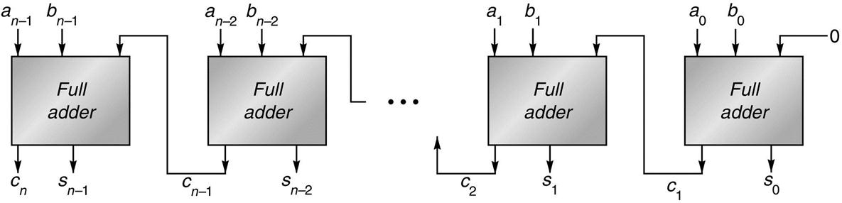
The carry-out of one full adder is connected to the carry-in of the adder for the next most-significant bit. The carries ripple from the least-significant bit (on the right) to the most-significant bit (on the left).
In general, the time a circuit takes to produce an output is proportional to the maximum number of logic levels through which a signal travels. However, determining the exact relationship between logic levels and timings is highly technology dependent. Therefore, when comparing adders we will simply compare the number of logic levels in each one. How many levels are there for a ripple-carry adder? It takes two levels to compute c1 from a0 and b0. Then it takes two more levels to compute c2 from c1, a1, b1, and so on, up to cn. So, there are a total of 2n levels. Typical values of n are 32 for integer arithmetic and 53 for double-precision floating point. The ripple-carry adder is the slowest adder, but also the cheapest. It can be built with only n simple cells, connected in a simple, regular way.
Because the ripple-carry adder is relatively slow compared with the designs discussed in Section J.8, you might wonder why it is used at all. In technologies like CMOS, even though ripple adders take time O(n), the constant factor is very small. In such cases short ripple adders are often used as building blocks in larger adders.
Radix-2 Multiplication and Division
The simplest multiplier computes the product of two unsigned numbers, one bit at a time, as illustrated in Figure J.2(a). The numbers to be multiplied are and , and they are placed in registers A and B, respectively. Register P is initially 0. Each multiply step has two parts:
- Multiply Step
- (i) If the least-significant bit of A is 1, then register B, containing , is added to P; otherwise,
 is added to P. The sum is placed back into P.
 - (ii) Registers P and A are shifted right, with the carry-out of the sum being moved into the high-order bit of P, the low-order bit of P being moved into register A, and the rightmost bit of A, which is not used in the rest of the algorithm, being shifted out.
- (i) If the least-significant bit of A is 1, then register B, containing
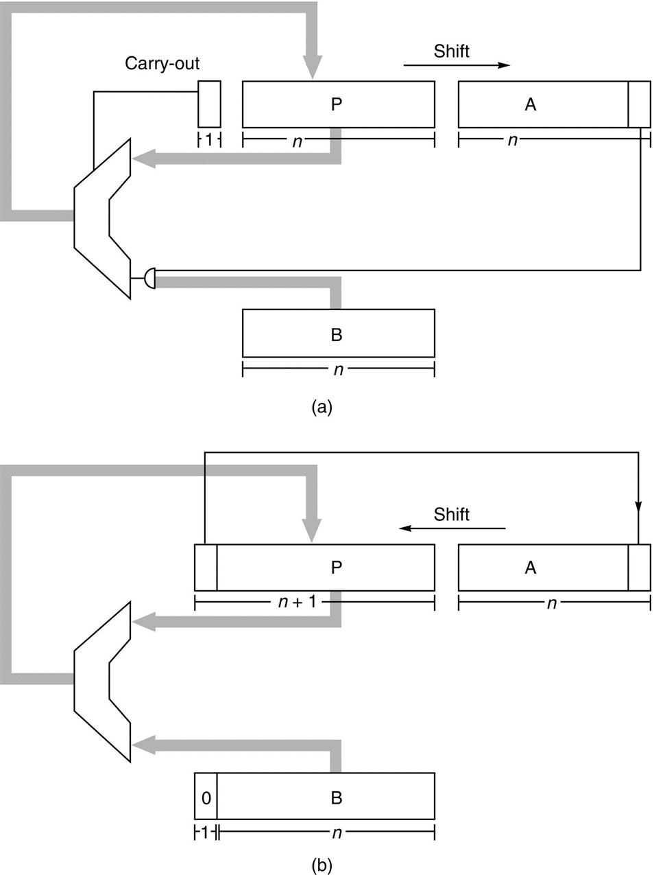
Each multiplication step consists of adding the contents of P to either B or 0 (depending on the low-order bit of A), replacing P with the sum, and then shifting both P and A one bit right. Each division step involves first shifting P and A one bit left, subtracting B from P, and, if the difference is nonnegative, putting it into P. If the difference is nonnegative, the low-order bit of A is set to 1.
After n steps, the product appears in registers P and A, with A holding the lower-order bits.
The simplest divider also operates on unsigned numbers and produces the quotient bits one at a time. A hardware divider is shown in Figure J.2(b). To compute a/b, put a in the A register, b in the B register, and 0 in the P register and then perform n divide steps. Each divide step consists of four parts:
- Divide Step
- (i) Shift the register pair (P,A) one bit left.
- (ii) Subtract the content of register B (which is
 ) from register P, putting the result back into P.
 - (iii) If the result of step 2 is negative, set the low-order bit of A to 0, otherwise to 1.
- (iv) If the result of step 2 is negative, restore the old value of P by adding the contents of register B back into P.
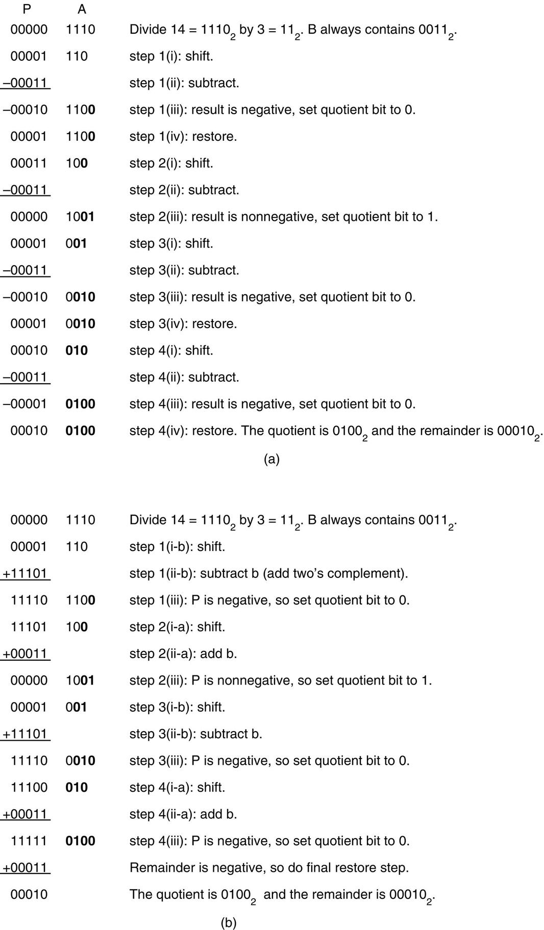
After repeating this process n times, the A register will contain the quotient, and the P register will contain the remainder. This algorithm is the binary version of the paper-and-pencil method; a numerical example is illustrated in Figure J.3(a).
Notice that the two block diagrams in Figure J.2 are very similar. The main difference is that the register pair (P,A) shifts right when multiplying and left when dividing. By allowing these registers to shift bidirectionally, the same hardware can be shared between multiplication and division.
The division algorithm illustrated in Figure J.3(a) is called restoring, because if subtraction by b yields a negative result, the P register is restored by adding b back in. The restoring algorithm has a variant that skips the restoring step and instead works with the resulting negative numbers. Each step of this nonrestoring algorithm has three parts:
After repeating this n times, the quotient is in A. If P is nonnegative, it is the remainder. Otherwise, it needs to be restored (i.e., add b), and then it will be the remainder. A numerical example is given in Figure J.3(b). Since steps (i-a) and (i-b) are the same, you might be tempted to perform this common step first, and then test the sign of P. That doesn’t work, since the sign bit can be lost when shifting.
The explanation for why the nonrestoring algorithm works is this. Let rk be the contents of the (P,A) register pair at step k, ignoring the quotient bits (which are simply sharing the unused bits of register A). In Figure J.3(a), initially A contains 14, so r0 = 14. At the end of the first step, r1 = 28, and so on. In the restoring algorithm, part (i) computes 2rk and then part (ii) 2rk − 2nb (2nb since b is subtracted from the left half). If 2rk − 2nb ≥ 0, both algorithms end the step with identical values in (P,A). If 2rk − 2nb < 0, then the restoring algorithm restores this to 2rk, and the next step begins by computing rres = 2(2rk) − 2nb. In the non-restoring algorithm, 2rk − 2nb is kept as a negative number, and in the next step rnonres = 2(2rk − 2nb) + 2nb = 4rk − 2nb = rres. Thus (P,A) has the same bits in both algorithms.
If a and b are unsigned n-bit numbers, hence in the range 0 ≤ a,b ≤ 2n − 1, then the multiplier in Figure J.2 will work if register P is n bits long. However, for division, P must be extended to n + 1 bits in order to detect the sign of P. Thus the adder must also have n + 1 bits.
Why would anyone implement restoring division, which uses the same hardware as nonrestoring division (the control is slightly different) but involves an extra addition? In fact, the usual implementation for restoring division doesn’t actually perform an add in step (iv). Rather, the sign resulting from the subtraction is tested at the output of the adder, and only if the sum is nonnegative is it loaded back into the P register.
As a final point, before beginning to divide, the hardware must check to see whether the divisor is 0.
Signed Numbers
There are four methods commonly used to represent signed n-bit numbers: sign magnitude, two’s complement, one’s complement, and biased. In the sign magnitude system, the high-order bit is the sign bit, and the low-order n − 1 bits are the magnitude of the number. In the two’s complement system, a number and its negative add up to 2n. In one’s complement, the negative of a number is obtained by complementing each bit (or, alternatively, the number and its negative add up to 2n − 1). In each of these three systems, nonnegative numbers are represented in the usual way. In a biased system, nonnegative numbers do not have their usual representation. Instead, all numbers are represented by first adding them to the bias and then encoding this sum as an ordinary unsigned number. Thus, a negative number k can be encoded as long as k + bias ≥ 0. A typical value for the bias is 2n − 1.
The most widely used system for representing integers, two’s complement, is the system we will use here. One reason for the popularity of two’s complement is that it makes signed addition easy: Simply discard the carry-out from the highorder bit. To add 5 + − 2, for example, add 01012 and 11102 to obtain 00112, resulting in the correct value of 3. A useful formula for the value of a two’s complement number  is
is
 J.2.3
J.2.3As an illustration of this formula, the value of 11012 as a 4-bit two’s complement number is − 1 · 23 + 1 · 22 + 0 · 21 + 1 · 20 = − 8 + 4 + 1 = − 3, confirming the result of the example above.
Overflow occurs when the result of the operation does not fit in the representation being used. For example, if unsigned numbers are being represented using 4 bits, then 6 = 01102 and 11 = 10112. Their sum (17) overflows because its binary equivalent (100012) doesn’t fit into 4 bits. For unsigned numbers, detecting overflow is easy; it occurs exactly when there is a carry-out of the most-significant bit. For two’s complement, things are trickier: Overflow occurs exactly when the carry into the high-order bit is different from the (to be discarded) carry-out of the high-order bit. In the example of 5 + − 2 above, a 1 is carried both into and out of the leftmost bit, avoiding overflow.
Negating a two’s complement number involves complementing each bit and then adding 1. For instance, to negate 00112, complement it to get 11002 and then add 1 to get 11012. Thus, to implement a − b using an adder, simply feed a and  (where is the number obtained by complementing each bit of b) into the adder and set the low-order, carry-in bit to 1. This explains why the rightmost adder in Figure J.1 is a full adder.
Multiplying two’s complement numbers is not quite as simple as adding them. The obvious approach is to convert both operands to be nonnegative, do an unsigned multiplication, and then (if the original operands were of opposite signs) negate the result. Although this is conceptually simple, it requires extra time and hardware. Here is a better approach: Suppose that we are multiplying a times b using the hardware shown in Figure J.2(a). Register A is loaded with the number a; B is loaded with b. Since the content of register B is always b, we will use B and b interchangeably. If B is potentially negative but A is nonnegative, the only change needed to convert the unsigned multiplication algorithm into a two’s complement one is to ensure that when P is shifted, it is shifted arithmetically; that is, the bit shifted into the high-order bit of P should be the sign bit of P (rather than the carry-out from the addition). Note that our n-bit-wide adder will now be adding n-bit two’s complement numbers between − 2n − 1 and 2n − 1 − 1.
Next, suppose a is negative. The method for handling this case is called Booth recoding. Booth recoding is a very basic technique in computer arithmetic and will play a key role in Section J.9. The algorithm on page J-4 computes a × b by examining the bits of a from least significant to most significant. For example, if a = 7 = 01112, then step (i) will successively add B, add B, add B, and add 0. Booth recoding “recodes” the number 7 as  , where
  represents − 1. This gives an alternative way to compute a × b, namely, successively subtract B, add 0, add 0, and add B. This is more complicated than the unsigned algorithm on page J-4, since it uses both addition and subtraction. The advantage shows up for negative values of a. With the proper recoding, we can treat a as though it were unsigned. For example, take a = − 4 = 11002. Think of 11002 as the unsigned number 12, and recode it as
  . If the multiplication algorithm is only iterated n times (n = 4 in this case), the high-order digit is ignored, and we end up subtracting 01002 = 4 times the multiplier—exactly the right answer. This suggests that multiplying using a recoded form of a will work equally well for both positive and negative numbers. And, indeed, to deal with negative values of a, all that is required is to sometimes subtract b from P, instead of adding either b or 0 to P. Here are the precise rules: If the initial content of A is
  , then at the ith multiply step the low-order bit of register A is ai, and step (i) in the multiplication algorithm becomes:
For the first step, when i = 0, take ai − 1 to be 0.
Example
When multiplying − 6 times − 5, what is the sequence of values in the (P,A) register pair?
Answer
See Figure J.4.
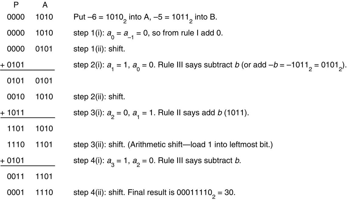
The four prior cases can be restated as saying that in the ith step you should add (ai − 1 − ai)B to P. With this observation, it is easy to verify that these rules work, because the result of all the additions is
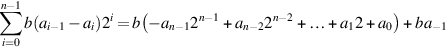
Using Equation J.2.3 (page J-8) together with a− 1 = 0, the right-hand side is seen to be the value of b × a as a two’s complement number.
The simplest way to implement the rules for Booth recoding is to extend the A register one bit to the right so that this new bit will contain ai − 1. Unlike the naive method of inverting any negative operands, this technique doesn’t require extra steps or any special casing for negative operands. It has only slightly more control logic. If the multiplier is being shared with a divider, there will already be the capability for subtracting b, rather than adding it. To summarize, a simple method for handling two’s complement multiplication is to pay attention to the sign of P when shifting it right, and to save the most recently shifted-out bit of A to use in deciding whether to add or subtract b from P.
Booth recoding is usually the best method for designing multiplication hardware that operates on signed numbers. For hardware that doesn’t directly implement it, however, performing Booth recoding in software or microcode is usually too slow because of the conditional tests and branches. If the hardware supports arithmetic shifts (so that negative b is handled correctly), then the following method can be used. Treat the multiplier a as if it were an unsigned number, and perform the first n − 1 multiply steps using the algorithm on page J-4. If a < 0 (in which case there will be a 1 in the low-order bit of the A register at this point), then subtract b from P; otherwise (a ≥ 0), neither add nor subtract. In either case, do a final shift (for a total of n shifts). This works because it amounts to multiplying b by 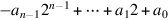 , which is the value of
  as a two’s complement number by Equation J.2.3. If the hardware doesn’t support arithmetic shift, then converting the operands to be nonnegative is probably the best approach.
Two final remarks: A good way to test a signed-multiply routine is to try − 2n − 1 × − 2n − 1, since this is the only case that produces a 2n − 1 bit result. Unlike multiplication, division is usually performed in hardware by converting the operands to be nonnegative and then doing an unsigned divide. Because division is substantially slower (and less frequent) than multiplication, the extra time used to manipulate the signs has less impact than it does on multiplication.
Systems Issues
When designing an instruction set, a number of issues related to integer arithmetic need to be resolved. Several of them are discussed here.
First, what should be done about integer overflow? This situation is complicated by the fact that detecting overflow differs depending on whether the operands are signed or unsigned integers. Consider signed arithmetic first. There are three approaches: Set a bit on overflow, trap on overflow, or do nothing on overflow. In the last case, software has to check whether or not an overflow occurred. The most convenient solution for the programmer is to have an enable bit. If this bit is turned on, then overflow causes a trap. If it is turned off, then overflow sets a bit (or, alternatively, have two different add instructions). The advantage of this approach is that both trapping and nontrapping operations require only one instruction. Furthermore, as we will see in Section J.7, this is analogous to how the IEEE floating-point standard handles floating-point overflow. Figure J.5 shows how some common machines treat overflow.
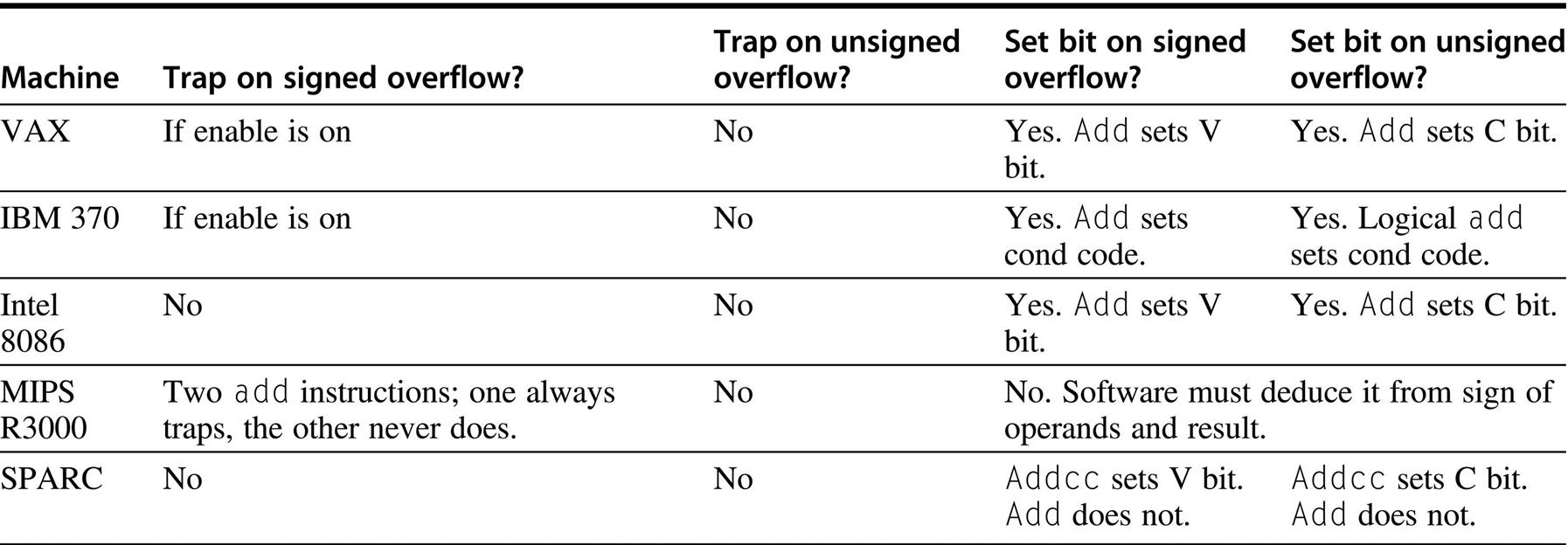
Both the 8086 and SPARC have an instruction that traps if the V bit is set, so the cost of trapping on overflow is one extra instruction.
What about unsigned addition? Notice that none of the architectures in Figure J.5 traps on unsigned overflow. The reason for this is that the primary use of unsigned arithmetic is in manipulating addresses. It is convenient to be able to subtract from an unsigned address by adding. For example, when n = 4, we can subtract 2 from the unsigned address 10 = 10102 by adding 14 = 11102. This generates an overflow, but we would not want a trap to be generated.
A second issue concerns multiplication. Should the result of multiplying two n-bit numbers be a 2n-bit result, or should multiplication just return the low-order n bits, signaling overflow if the result doesn’t fit in n bits? An argument in favor of an n-bit result is that in virtually all high-level languages, multiplication is an operation in which arguments are integer variables and the result is an integer variable of the same type. Therefore, compilers won’t generate code that utilizes a double-precision result. An argument in favor of a 2n-bit result is that it can be used by an assembly language routine to substantially speed up multiplication of multiple-precision integers (by about a factor of 3).
A third issue concerns machines that want to execute one instruction every cycle. It is rarely practical to perform a multiplication or division in the same amount of time that an addition or register-register move takes. There are three possible approaches to this problem. The first is to have a single-cycle multiply-step instruction. This might do one step of the Booth algorithm. The second approach is to do integer multiplication in the floating-point unit and have it be part of the floating-point instruction set. (This is what DLX does.) The third approach is to have an autonomous unit in the CPU do the multiplication. In this case, the result either can be guaranteed to be delivered in a fixed number of cycles—and the compiler charged with waiting the proper amount of time—or there can be an interlock. The same comments apply to division as well. As examples, the original SPARC had a multiply-step instruction but no divide-step instruction, while the MIPS R3000 has an autonomous unit that does multiplication and division (newer versions of the SPARC architecture added an integer multiply instruction). The designers of the HP Precision Architecture did an especially thorough job of analyzing the frequency of the operands for multiplication and division, and they based their multiply and divide steps accordingly. (See Magenheimer et al. [1988] for details.)
The final issue involves the computation of integer division and remainder for negative numbers. For example, what is − 5 DIV 3 and − 5 MOD 3? When computing x DIV y and x MOD y, negative values of x occur frequently enough to be worth some careful consideration. (On the other hand, negative values of y are quite rare.) If there are built-in hardware instructions for these operations, they should correspond to what high-level languages specify. Unfortunately, there is no agreement among existing programming languages. See Figure J.6.
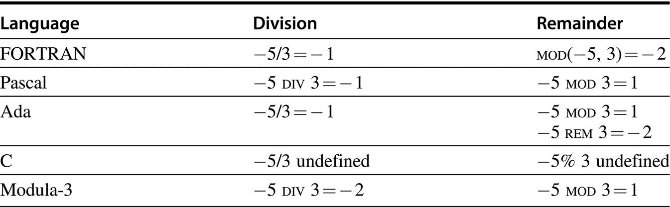
One definition for these expressions stands out as clearly superior, namely, x DIV y = ⌊x/y⌋, so that 5 DIV 3 = 1 and − 5 DIV 3 = − 2. And MOD should satisfy x = (x DIV y) × y + x MOD y, so that x MOD y ≥ 0. Thus, 5 MOD 3 = 2, and − 5 MOD 3 = 1. Some of the many advantages of this definition are as follows:
- 1. A calculation to compute an index into a hash table of size N can use MOD N and be guaranteed to produce a valid index in the range from 0 to N − 1.
- 2. In graphics, when converting from one coordinate system to another, there is no “glitch” near 0. For example, to convert from a value x expressed in a system that uses 100 dots per inch to a value y on a bitmapped display with 70 dots per inch, the formula y = (70 × x) DIV 100 maps one or two x coordinates into each y coordinate. But if DIV were defined as in Pascal to be x/y rounded to 0, then 0 would have three different points (− 1, 0, 1) mapped into it.
- 3. x MOD 2k is the same as performing a bitwise AND with a mask of k bits, and x DIV 2k is the same as doing a k-bit arithmetic right shift.
Finally, a potential pitfall worth mentioning concerns multiple-precision addition. Many instruction sets offer a variant of the add instruction that adds three operands: two n-bit numbers together with a third single-bit number. This third number is the carry from the previous addition. Since the multiple-precision number will typically be stored in an array, it is important to be able to increment the array pointer without destroying the carry bit.
J.3 Floating Point
Many applications require numbers that aren’t integers. There are a number of ways that nonintegers can be represented. One is to use fixed point; that is, use integer arithmetic and simply imagine the binary point somewhere other than just to the right of the least-significant digit. Adding two such numbers can be done with an integer add, whereas multiplication requires some extra shifting. Other representations that have been proposed involve storing the logarithm of a number and doing multiplication by adding the logarithms, or using a pair of integers (a,b) to represent the fraction a/b. However, only one noninteger representation has gained widespread use, and that is floating point. In this system, a computer word is divided into two parts, an exponent and a significand. As an example, an exponent of − 3 and a significand of 1.5 might represent the number 1.5 × 2− 3 = 0.1875. The advantages of standardizing a particular representation are obvious. Numerical analysts can build up high-quality software libraries, computer designers can develop techniques for implementing high-performance hardware, and hardware vendors can build standard accelerators. Given the predominance of the floating-point representation, it appears unlikely that any other representation will come into widespread use.
The semantics of floating-point instructions are not as clear-cut as the semantics of the rest of the instruction set, and in the past the behavior of floating-point operations varied considerably from one computer family to the next. The variations involved such things as the number of bits allocated to the exponent and significand, the range of exponents, how rounding was carried out, and the actions taken on exceptional conditions like underflow and overflow. Computer architecture books used to dispense advice on how to deal with all these details, but fortunately this is no longer necessary. That’s because the computer industry is rapidly converging on the format specified by IEEE standard 754-1985 (also an international standard, IEC 559). The advantages of using a standard variant of floating point are similar to those for using floating point over other noninteger representations.
IEEE arithmetic differs from many previous arithmetics in the following major ways:
- 1. When rounding a “halfway” result to the nearest floating-point number, it picks the one that is even.
- 2. It includes the special values NaN, ∞, and − ∞.
- 3. It uses denormal numbers to represent the result of computations whose value is less than
 .
. - 4. It rounds to nearest by default, but it also has three other rounding modes.
- 5. It has sophisticated facilities for handling exceptions.
To elaborate on (1), note that when operating on two floating-point numbers, the result is usually a number that cannot be exactly represented as another floating-point number. For example, in a floating-point system using base 10 and two significant digits, 6.1 × 0.5 = 3.05. This needs to be rounded to two digits. Should it be rounded to 3.0 or 3.1? In the IEEE standard, such halfway cases are rounded to the number whose low-order digit is even. That is, 3.05 rounds to 3.0, not 3.1. The standard actually has four rounding modes. The default is round to nearest, which rounds ties to an even number as just explained. The other modes are round toward 0, round toward + ∞, and round toward − ∞.
We will elaborate on the other differences in following sections. For further reading, see IEEE [1985], Cody et al. [1984], and Goldberg [1991].
Special Values and Denormals
Probably the most notable feature of the standard is that by default a computation continues in the face of exceptional conditions, such as dividing by 0 or taking the square root of a negative number. For example, the result of taking the square root of a negative number is a NaN (Not a Number), a bit pattern that does not represent an ordinary number. As an example of how NaNs might be useful, consider the code for a zero finder that takes a function F as an argument and evaluates F at various points to determine a zero for it. If the zero finder accidentally probes outside the valid values for F, then F may well cause an exception. Writing a zero finder that deals with this case is highly language and operating-system dependent, because it relies on how the operating system reacts to exceptions and how this reaction is mapped back into the programming language. In IEEE arithmetic it is easy to write a zero finder that handles this situation and runs on many different systems. After each evaluation of F, it simply checks to see whether F has returned a NaN; if so, it knows it has probed outside the domain of F.
In IEEE arithmetic, if the input to an operation is a NaN, the output is NaN (e.g., 3 + NaN = NaN). Because of this rule, writing floating-point subroutines that can accept NaN as an argument rarely requires any special case checks. For example, suppose that arccos is computed in terms of arctan, using the formula  . If arctan handles an argument of NaN properly, arccos will automatically do so, too. That’s because if x is a NaN, 1 + x, 1 − x, (1 + x)/(1 − x), and
  will also be NaNs. No checking for NaNs is required.
While the result of  is a NaN, the result of 1/0 is not a NaN, but + ∞, which is another special value. The standard defines arithmetic on infinities (there are both + ∞ and − ∞) using rules such as 1/∞ = 0. The formula illustrates how infinity arithmetic can be used. Since arctan x asymptotically approaches π/2 as x approaches ∞, it is natural to define arctan(∞) = π/2, in which case arccos(− 1) will automatically be computed correctly as 2 arctan(∞) = π.
The final kind of special values in the standard are denormal numbers. In many floating-point systems, if Emin is the smallest exponent, a number less than cannot be represented, and a floating-point operation that results in a number less than this is simply flushed to 0. In the IEEE standard, on the other hand, numbers less than are represented using significands less than 1. This is called gradual underflow. Thus, as numbers decrease in magnitude below  , they gradually lose their significance and are only represented by 0 when all their significance has been shifted out. For example, in base 10 with four significant figures, let
  . Then, x/10 will be rounded to
  , having lost a digit of precision. Similarly x/100 rounds to
  , and x/1000 to
  , while x/10000 is finally small enough to be rounded to 0. Denormals make dealing with small numbers more predictable by maintaining familiar properties such as x = y ⇔ x − y = 0. For example, in a flush-to-zero system (again in base 10 with four significant digits), if
  and
and  , then
  , which flushes to zero. So even though x ≠ y, the computed value of x − y = 0. This never happens with gradual underflow. In this example, is a denormal number, and so the computation of x − y is exact.
Representation of Floating-Point Numbers
Let us consider how to represent single-precision numbers in IEEE arithmetic. Single-precision numbers are stored in 32 bits: 1 for the sign, 8 for the exponent, and 23 for the fraction. The exponent is a signed number represented using the bias method (see the subsection “Signed Numbers,” page J-7) with a bias of 127. The term biased exponent refers to the unsigned number contained in bits 1 through 8, and unbiased exponent (or just exponent) means the actual power to which 2 is to be raised. The fraction represents a number less than 1, but the significand of the floating-point number is 1 plus the fraction part. In other words, if e is the biased exponent (value of the exponent field) and f is the value of the fraction field, the number being represented is 1. f × 2e − 127.
Example
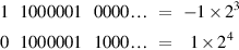
What single-precision number does the following 32-bit word represent?

Answer
Considered as an unsigned number, the exponent field is 129, making the value of the exponent 129 − 127 = 2. The fraction part is .012 = .25, making the significand 1.25. Thus, this bit pattern represents the number − 1.25 × 22 = − 5.
The fractional part of a floating-point number (.25 in the example above) must not be confused with the significand, which is 1 plus the fractional part. The leading 1 in the significand 1.f does not appear in the representation; that is, the leading bit is implicit. When performing arithmetic on IEEE format numbers, the fraction part is usually unpacked, which is to say the implicit 1 is made explicit.
Figure J.7 summarizes the parameters for single (and other) precisions. It shows the exponents for single precision to range from − 126 to 127; accordingly, the biased exponents range from 1 to 254. The biased exponents of 0 and 255 are used to represent special values. This is summarized in Figure J.8. When the biased exponent is 255, a zero fraction field represents infinity, and a nonzero fraction field represents a NaN. Thus, there is an entire family of NaNs. When the biased exponent and the fraction field are 0, then the number represented is 0. Because of the implicit leading 1, ordinary numbers always have a significand greater than or equal to 1. Thus, a special convention such as this is required to represent 0. Denormalized numbers are implemented by having a word with a zero exponent field represent the number  .
.
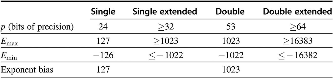
The first row gives the number of bits in the significand. The blanks are unspecified parameters.
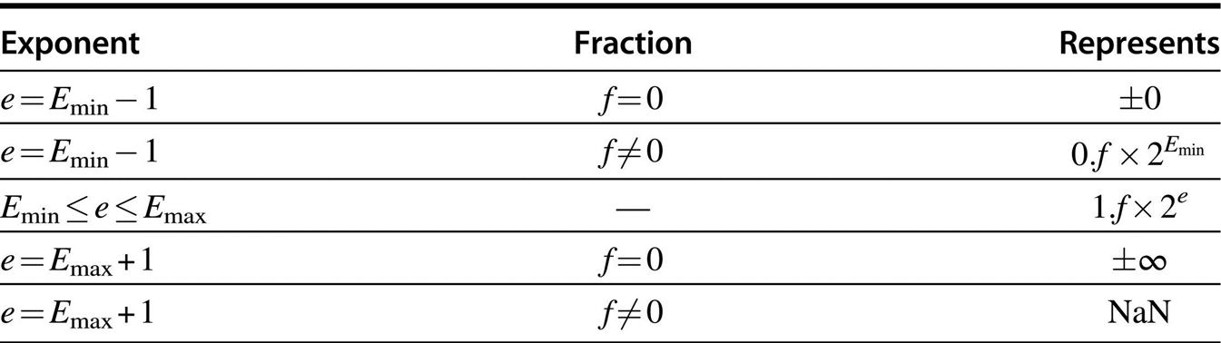
When the exponent of a number falls outside the range Emin ≤ e ≤ Emax, then that number has a special interpretation as indicated in the table.
The primary reason why the IEEE standard, like most other floating-point formats, uses biased exponents is that it means nonnegative numbers are ordered in the same way as integers. That is, the magnitude of floating-point numbers can be compared using an integer comparator. Another (related) advantage is that 0 is represented by a word of all 0s. The downside of biased exponents is that adding them is slightly awkward, because it requires that the bias be subtracted from their sum.
J.4 Floating-Point Multiplication
The simplest floating-point operation is multiplication, so we discuss it first. A binary floating-point number x is represented as a significand and an exponent, x = s × 2e. The formula

shows that a floating-point multiply algorithm has several parts. The first part multiplies the significands using ordinary integer multiplication. Because floating-point numbers are stored in sign magnitude form, the multiplier need only deal with unsigned numbers (although we have seen that Booth recoding handles signed two’s complement numbers painlessly). The second part rounds the result. If the significands are unsigned p-bit numbers (e.g., p = 24 for single precision), then the product can have as many as 2p bits and must be rounded to a p-bit number. The third part computes the new exponent. Because exponents are stored with a bias, this involves subtracting the bias from the sum of the biased exponents.
Example
How does the multiplication of the single-precision numbers
proceed in binary?
Answer
When unpacked, the significands are both 1.0, their product is 1.0, and so the result is of the form:

To compute the exponent, use the formula:

From Figure J.7, the bias is 127 = 011111112, so in two’s complement − 127 is 100000012. Thus, the biased exponent of the product is

Since this is 134 decimal, it represents an exponent of 134 − bias = 134 − 127, as expected.
The interesting part of floating-point multiplication is rounding. Some of the different cases that can occur are illustrated in Figure J.9. Since the cases are similar in all bases, the figure uses human-friendly base 10, rather than base 2.
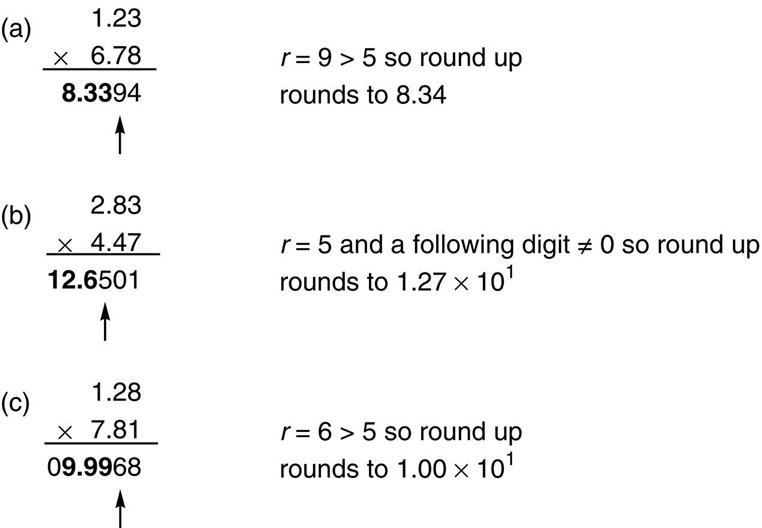
Using base 10 and p = 3, parts (a) and (b) illustrate that the result of a multiplication can have either 2p − 1 or 2p digits; hence, the position where a 1 is added when rounding up (just left of the arrow) can vary. Part (c) shows that rounding up can cause a carry-out.
In the figure, p = 3, so the final result must be rounded to three significant digits. The three most-significant digits are in boldface. The fourth most-significant digit (marked with an arrow) is the round digit, denoted by r.
If the round digit is less than 5, then the bold digits represent the rounded result. If the round digit is greater than 5 (as in part (a)), then 1 must be added to the least-significant bold digit. If the round digit is exactly 5 (as in part (b)), then additional digits must be examined to decide between truncation or incrementing by 1. It is only necessary to know if any digits past 5 are nonzero. In the algorithm below, this will be recorded in a sticky bit. Comparing parts (a) and (b) in the figure shows that there are two possible positions for the round digit (relative to the least-significant digit of the product). Case (c) illustrates that, when adding 1 to the least-significant bold digit, there may be a carry-out. When this happens, the final significand must be 10.0.
There is a straightforward method of handling rounding using the multiplier of Figure J.2 (page J-4) together with an extra sticky bit. If p is the number of bits in the significand, then the A, B, and P registers should be p bits wide. Multiply the two significands to obtain a 2p-bit product in the (P,A) registers (see Figure J.10). During the multiplication, the first p − 2 times a bit is shifted into the A register, OR it into the sticky bit. This will be used in halfway cases. Let s represent the sticky bit, g (for guard) the most-significant bit of A, and r (for round) the second most-significant bit of A. There are two cases:
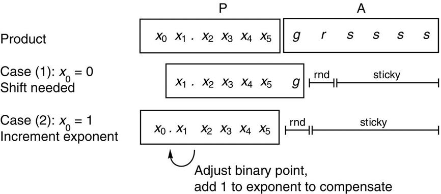
The top line shows the contents of the P and A registers after multiplying the significands, with p = 6. In case (1), the leading bit is 0, and so the P register must be shifted. In case (2), the leading bit is 1, no shift is required, but both the exponent and the round and sticky bits must be adjusted. The sticky bit is the logical OR of the bits marked s.
Now if r = 0, P is the correctly rounded product. If r = 1 and s = 1, then P + 1 is the product (where by P + 1 we mean adding 1 to the least-significant bit of P).
If r = 1 and s = 0, we are in a halfway case and round up according to the least-significant bit of P. As an example, apply the decimal version of these rules to Figure J.9(b). After the multiplication, P = 126 and A = 501, with g = 5, r = 0 and s = 1. Since the high-order digit of P is nonzero, case (2) applies and r := g, so that r = 5, as the arrow indicates in Figure J.9. Since r = 5, we could be in a halfway case, but s = 1 indicates that the result is in fact slightly over 1/2, so add 1 to P to obtain the correctly rounded product.
The precise rules for rounding depend on the rounding mode and are given in Figure J.11. Note that P is nonnegative, that is, it contains the magnitude of the result. A good discussion of more efficient ways to implement rounding is in Santoro, Bewick, and Horowitz [1989].
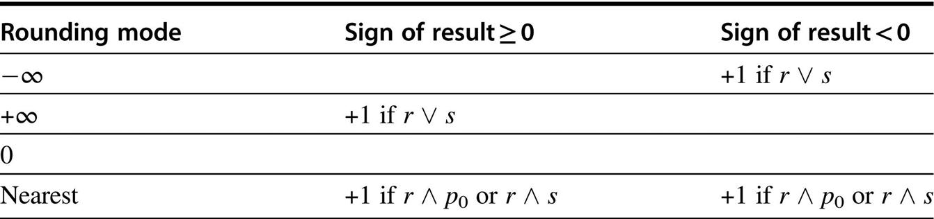
Let S be the magnitude of the preliminary result. Blanks mean that the p most-significant bits of S are the actual result bits. If the condition listed is true, add 1 to the pth most-significant bit of S. The symbols r and s represent the round and sticky bits, while p0 is the pth most-significant bit of S.
Example
In binary with p = 4, show how the multiplication algorithm computes the product − 5 × 10 in each of the four rounding modes.
Answer
In binary, − 5 is − 1.0102 × 22 and 10 = 1.0102 × 23. Applying the integer multiplication algorithm to the significands gives 011001002, so P = 01102, A = 01002, g = 0, r = 1, and s = 0. The high-order bit of P is 0, so case (1) applies. Thus, P becomes 11002, and since the result is negative, Figure J.11 gives:
| round to − ∞ | 11012 | add 1 since r ∨ s = 1 / 0 = TRUE | |
| round to + ∞ | 11002 | ||
| round to 0 | 11002 | ||
| round to nearest | 11002 | no add since | r ∧ p0 = 1 ∧ 0 = FALSE and r ∧ s = 1 ∧ 0 = FALSE |
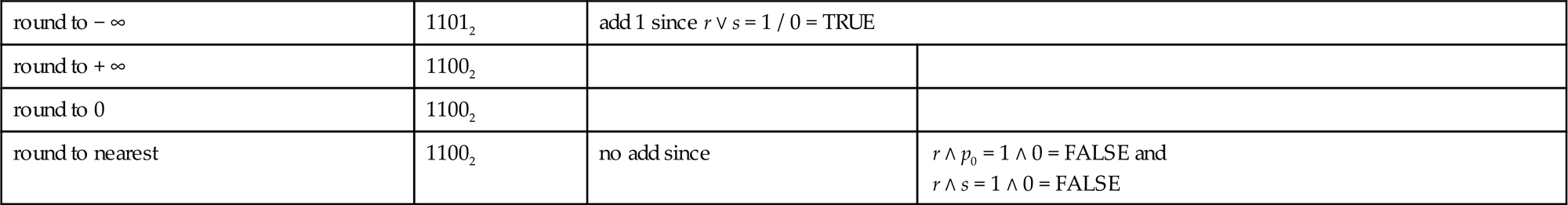
The exponent is 2 + 3 = 5, so the result is − 1.1002 × 25 = − 48, except when rounding to − ∞, in which case it is − 1.1012 × 25 = − 52.
Overflow occurs when the rounded result is too large to be represented. In single precision, this occurs when the result has an exponent of 128 or higher. If e1 and e2 are the two biased exponents, then 1 ≤ ei ≤ 254, and the exponent calculation e1 + e2 − 127 gives numbers between 1 + 1 − 127 and 254 + 254 − 127, or between − 125 and 381. This range of numbers can be represented using 9 bits. So one way to detect overflow is to perform the exponent calculations in a 9-bit adder (see Exercise J.12). Remember that you must check for overflow after rounding—the example in Figure J.9(c) shows that this can make a difference.
Denormals
Checking for underflow is somewhat more complex because of denormals. In single precision, if the result has an exponent less than − 126, that does not necessarily indicate underflow, because the result might be a denormal number. For example, the product of (1 × 2− 64) with (1 × 2− 65) is 1 × 2− 129, and − 129 is below the legal exponent limit. But this result is a valid denormal number, namely, 0.125 × 2− 126. In general, when the unbiased exponent of a product dips below − 126, the resulting product must be shifted right and the exponent incremented until the exponent reaches − 126. If this process causes the entire significand to be shifted out, then underflow has occurred. The precise definition of underflow is somewhat subtle—see Section J.7 for details.
When one of the operands of a multiplication is denormal, its significand will have leading zeros, and so the product of the significands will also have leading zeros. If the exponent of the product is less than − 126, then the result is denormal, so right-shift and increment the exponent as before. If the exponent is greater than − 126, the result may be a normalized number. In this case, left-shift the product (while decrementing the exponent) until either it becomes normalized or the exponent drops to − 126.
Denormal numbers present a major stumbling block to implementing floating-point multiplication, because they require performing a variable shift in the multiplier, which wouldn’t otherwise be needed. Thus, high-performance, floating-point multipliers often do not handle denormalized numbers, but instead trap, letting software handle them. A few practical codes frequently underflow, even when working properly, and these programs will run quite a bit slower on systems that require denormals to be processed by a trap handler.
So far we haven’t mentioned how to deal with operands of zero. This can be handled by either testing both operands before beginning the multiplication or testing the product afterward. If you test afterward, be sure to handle the case 0 × ∞ properly: This results in NaN, not 0. Once you detect that the result is 0, set the biased exponent to 0. Don’t forget about the sign. The sign of a product is the XOR of the signs of the operands, even when the result is 0.
Precision of Multiplication
In the discussion of integer multiplication, we mentioned that designers must decide whether to deliver the low-order word of the product or the entire product. A similar issue arises in floating-point multiplication, where the exact product can be rounded to the precision of the operands or to the next higher precision. In the case of integer multiplication, none of the standard high-level languages contains a construct that would generate a “single times single gets double” instruction. The situation is different for floating point. Many languages allow assigning the product of two single-precision variables to a double-precision one, and the construction can also be exploited by numerical algorithms. The best-known case is using iterative refinement to solve linear systems of equations.
J.5 Floating-Point Addition
Typically, a floating-point operation takes two inputs with p bits of precision and returns a p-bit result. The ideal algorithm would compute this by first performing the operation exactly, and then rounding the result to p bits (using the current rounding mode). The multiplication algorithm presented in the previous section follows this strategy. Even though hardware implementing IEEE arithmetic must return the same result as the ideal algorithm, it doesn’t need to actually perform the ideal algorithm. For addition, in fact, there are better ways to proceed. To see this, consider some examples.
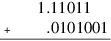
First, the sum of the binary 6-bit numbers 1.100112 and 1.100012 × 2− 5: When the summands are shifted so they have the same exponent, this is
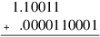
Using a 6-bit adder (and discarding the low-order bits of the second addend) gives

The first discarded bit is 1. This isn’t enough to decide whether to round up. The rest of the discarded bits, 0001, need to be examined. Or, actually, we just need to record whether any of these bits are nonzero, storing this fact in a sticky bit just as in the multiplication algorithm. So, for adding two p-bit numbers, a p-bit adder is sufficient, as long as the first discarded bit (round) and the OR of the rest of the bits (sticky) are kept. Then Figure J.11 can be used to determine if a roundup is necessary, just as with multiplication. In the example above, sticky is 1, so a roundup is necessary. The final sum is 1.101012.
Here’s another example:
A 6-bit adder gives:

Because of the carry-out on the left, the round bit isn’t the first discarded bit; rather, it is the low-order bit of the sum (1). The discarded bits, 01, are OR’ed together to make sticky. Because round and sticky are both 1, the high-order 6 bits of the sum, 10.00102, must be rounded up for the final answer of 10.00112.
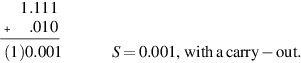
Next, consider subtraction and the following example:
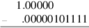
The simplest way of computing this is to convert − .000001011112 to its two’s complement form, so the difference becomes a sum:
Computing this sum in a 6-bit adder gives:

Because the top bits canceled, the first discarded bit (the guard bit) is needed to fill in the least-significant bit of the sum, which becomes 0.1111102, and the second discarded bit becomes the round bit. This is analogous to case (1) in the multiplication algorithm (see page J-19). The round bit of 1 isn’t enough to decide whether to round up. Instead, we need to OR all the remaining bits (0001) into a sticky bit. In this case, sticky is 1, so the final result must be rounded up to 0.111111. This example shows that if subtraction causes the most-significant bit to cancel, then one guard bit is needed. It is natural to ask whether two guard bits are needed for the case when the two most-significant bits cancel. The answer is no, because if x and y are so close that the top two bits of x − y cancel, then x − y will be exact, so guard bits aren’t needed at all.
To summarize, addition is more complex than multiplication because, depending on the signs of the operands, it may actually be a subtraction. If it is an addition, there can be carry-out on the left, as in the second example. If it is subtraction, there can be cancellation, as in the third example. In each case, the position of the round bit is different. However, we don’t need to compute the exact sum and then round. We can infer it from the sum of the high-order p bits together with the round and sticky bits.
The rest of this section is devoted to a detailed discussion of the floatingpoint addition algorithm. Let a1 and a2 be the two numbers to be added. The notations ei and si are used for the exponent and significand of the addends ai. This means that the floating-point inputs have been unpacked and that si has an explicit leading bit. To add a1 and a2, perform these eight steps:
- 1. If e1 < e2, swap the operands. This ensures that the difference of the exponents satisfies d = e1 − e2 ≥ 0. Tentatively set the exponent of the result to e1.
- 2. If the signs of a1 and a2 differ, replace s2 by its two’s complement.
- 3. Place s2 in a p-bit register and shift it d = e1 − e2 places to the right (shifting in 1’s if s2 was complemented in the previous step). From the bits shifted out, set g to the most-significant bit, set r to the next most-significant bit, and set sticky to the OR of the rest.
- 4. Compute a preliminary significand S = s1 + s2 by adding s1 to the p-bit register containing s2. If the signs of a1 and a2 are different, the most-significant bit of S is 1, and there was no carry-out, then S is negative. Replace S with its two’s complement. This can only happen when d = 0.
- 5. Shift S as follows. If the signs of a1 and a2 are the same and there was a carryout in step 4, shift S right by one, filling in the high-order position with 1 (the carry-out). Otherwise, shift it left until it is normalized. When left-shifting, on the first shift fill in the low-order position with the g bit. After that, shift in zeros. Adjust the exponent of the result accordingly.
- 6. Adjust r and s. If S was shifted right in step 5, set r := low-order bit of S before shifting and s := g OR r OR s. If there was no shift, set r := g, s := r OR s. If there was a single left shift, don’t change r and s. If there were two or more left shifts, r := 0, s := 0. (In the last case, two or more shifts can only happen when a1 and a2 have opposite signs and the same exponent, in which case the computation s1 + s2 in step 4 will be exact.)
- 7. Round S using Figure J.11; namely, if a table entry is nonempty, add 1 to the low-order bit of S. If rounding causes carry-out, shift S right and adjust the exponent. This is the significand of the result.
- 8. Compute the sign of the result. If a1 and a2 have the same sign, this is the sign of the result. If a1 and a2 have different signs, then the sign of the result depends on which of a1 or a2 is negative, whether there was a swap in step 1, and whether S was replaced by its two’s complement in step 4. See Figure J.12.
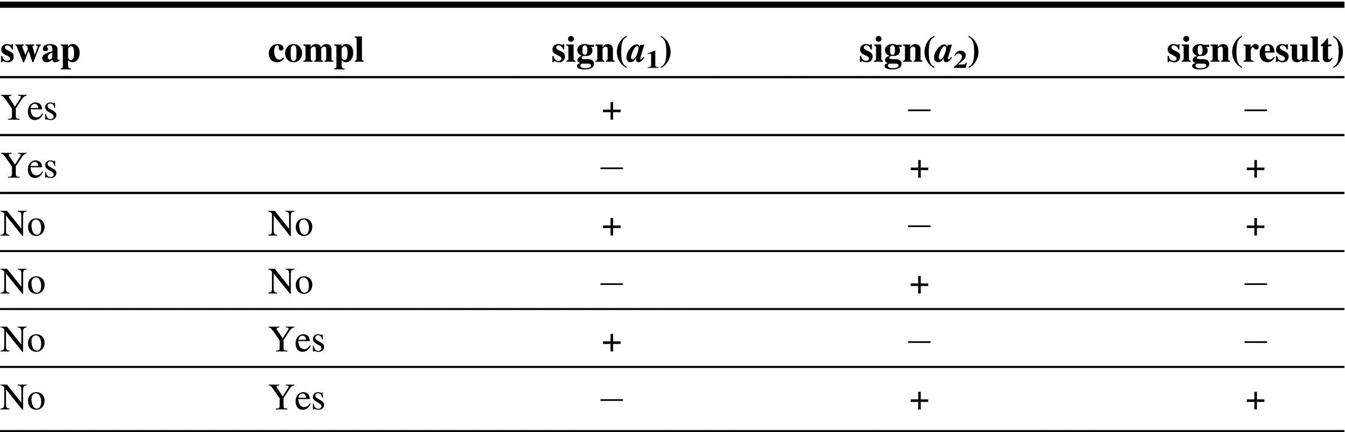
The swap column refers to swapping the operands in step 1, while the compl column refers to performing a two’s complement in step 4. Blanks are “don’t care.”
Example
Use the algorithm to compute the sum (− 1.0012 × 2− 2) + (− 1.1112 × 20).
Answer
s1 = 1.001, e1 = − 2, s2 = 1.111, e2 = 0
- 1. e1 < e2, so swap. d = 2. Tentative exp = 0.
- 2. Signs of both operands negative, don’t negate s2.
- 3. Shift s2 (1.001 after swap) right by 2, giving s2 = .010, g = 0, r = 1, s = 0.
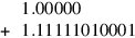
- 4.
- 5. Carry-out, so shift S right, S = 1.000, exp = exp + 1, so exp = 1.
- 6. r = low-order bit of sum = 1, s = g ∨ r ∨ s = 0 ∨ 1 ∨ 0 = 1.
- 7. r AND s = TRUE, so Figure J.11 says round up, S = S + 1 or S = 1.001.
- 8. Both signs negative, so sign of result is negative. Final answer: − S × 2exp = 1.0012 × 21.
Example
Use the algorithm to compute the sum (− 1.0102) + 1.1002.
Answer
s1 = 1.010, e1 = 0, s2 = 1.100, e2 = 0
- 1. No swap, d = 0, tentative exp = 0.
- 2. Signs differ, replace s2 with 0.100.
- 3. d = 0, so no shift. r = g = s = 0.
- 4.
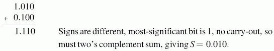
- 5. Shift left twice, so S = 1.000, exp = exp − 2, or exp = − 2.
- 6. Two left shifts, so r = g = s = 0.
- 7. No addition required for rounding.
- 8. Answer is sign × S × 2exp or sign × 1.000 × 2− 2. Get sign from Figure J.12. Since complement but no swap and sign(a1) is −, the sign of the sum is +. Thus, the answer = 1.0002 × 2− 2.
Speeding Up Addition
Let’s estimate how long it takes to perform the algorithm above. Step 2 may require an addition, step 4 requires one or two additions, and step 7 may require an addition. If it takes T time units to perform a p-bit add (where p = 24 for single precision, 53 for double), then it appears the algorithm will take at least 4 T time units. But that is too pessimistic. If step 4 requires two adds, then a1 and a2 have the same exponent and different signs, but in that case the difference is exact, so no roundup is required in step 7. Thus, only three additions will ever occur. Similarly, it appears that a variable shift may be required both in step 3 and step 5. But if |e1 − e2| ≤ 1, then step 3 requires a right shift of at most one place, so only step 5 needs a variable shift. And, if |e1 − e2| > 1, then step 3 needs a variable shift, but step 5 will require a left shift of at most one place. So only a single variable shift will be performed. Still, the algorithm requires three sequential adds, which, in the case of a 53-bit double-precision significand, can be rather time consuming.
A number of techniques can speed up addition. One is to use pipelining. The “Putting It All Together” section gives examples of how some commercial chips pipeline addition. Another method (used on the Intel 860 [Kohn and Fu 1989]) is to perform two additions in parallel. We now explain how this reduces the latency from 3T to T.
There are three cases to consider. First, suppose that both operands have the same sign. We want to combine the addition operations from steps 4 and 7. The position of the high-order bit of the sum is not known ahead of time, because the addition in step 4 may or may not cause a carry-out. Both possibilities are accounted for by having two adders. The first adder assumes the add in step 4 will not result in a carry-out. Thus, the values of r and s can be computed before the add is actually done. If r and s indicate that a roundup is necessary, the first adder will compute S = s1 + s2 + 1, where the notation + 1 means adding 1 at the position of the least-significant bit of s1. This can be done with a regular adder by setting the low-order carry-in bit to 1. If r and s indicate no roundup, the adder computes S = s1 + s2 as usual. One extra detail: When r = 1, s = 0, you will also need to know the low-order bit of the sum, which can also be computed in advance very quickly. The second adder covers the possibility that there will be carry-out. The values of r and s and the position where the roundup 1 is added are different from above, but again they can be quickly computed in advance. It is not known whether there will be a carry-out until after the add is actually done, but that doesn’t matter. By doing both adds in parallel, one adder is guaranteed to reduce the correct answer.
The next case is when a1 and a2 have opposite signs but the same exponent. The sum a1 + a2 is exact in this case (no roundup is necessary) but the sign isn’t known until the add is completed. So don’t compute the two’s complement (which requires an add) in step 2, but instead compute  and
and  in parallel. The first sum has the result of simultaneously complementing s1 and computing the sum, resulting in s2 − s1. The second sum computes s1 − s2. One of these will be nonnegative and hence the correct final answer. Once again, all the additions are done in one step using two adders operating in parallel.
The last case, when a1 and a2 have opposite signs and different exponents, is more complex. If |e1 − e2| > 1, the location of the leading bit of the difference is in one of two locations, so there are two cases just as in addition. When |e1 − e2| = 1, cancellation is possible and the leading bit could be almost anywhere. However, only if the leading bit of the difference is in the same position as the leading bit of s1 could a roundup be necessary. So one adder assumes a roundup, and the other assumes no roundup. Thus, the addition of step 4 and the rounding of step 7 can be combined. However, there is still the problem of the addition in step 2!
To eliminate this addition, consider the following diagram of step 4:
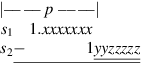
If the bits marked z are all 0, then the high-order p bits of S = s1 − s2 can be computed as . If at least one of the z bits is 1, use  . So s1 − s2 can be computed with one addition. However, we still don’t know g and r for the two’s complement of s2, which are needed for rounding in step 7.
To compute s1 − s2 and get the proper g and r bits, combine steps 2 and 4 as follows. Don’t complement s2 in step 2. Extend the adder used for computing S two bits to the right (call the extended sum S′). If the preliminary sticky bit (computed in step 3) is 1, compute  , where s1′ has two 0 bits tacked onto the right, and s2′ has preliminary g and r appended. If the sticky bit is 0, compute
  . Now the two low-order bits of S′ have the correct values of g and r (the sticky bit was already computed properly in step 3). Finally, this modification can be combined with the modification that combines the addition from steps 4 and 7 to provide the final result in time T, the time for one addition.
A few more details need to be considered, as discussed in Santoro, Bewick, and Horowitz [1989] and Exercise J.17. Although the Santoro paper is aimed at multiplication, much of the discussion applies to addition as well. Also relevant is Exercise J.19, which contains an alternative method for adding signed magnitude numbers.
Denormalized Numbers
Unlike multiplication, for addition very little changes in the preceding description if one of the inputs is a denormal number. There must be a test to see if the exponent field is 0. If it is, then when unpacking the significand there will not be a leading 1. By setting the biased exponent to 1 when unpacking a denormal, the algorithm works unchanged.
To deal with denormalized outputs, step 5 must be modified slightly. Shift S until it is normalized, or until the exponent becomes Emin (that is, the biased exponent becomes 1). If the exponent is Emin and, after rounding, the high-order bit of S is 1, then the result is a normalized number and should be packed in the usual way, by omitting the 1. If, on the other hand, the high-order bit is 0, the result is denormal. When the result is unpacked, the exponent field must be set to 0. Section J.7 discusses the exact rules for detecting underflow.
Incidentally, detecting overflow is very easy. It can only happen if step 5 involves a shift right and the biased exponent at that point is bumped up to 255 in single precision (or 2047 for double precision), or if this occurs after rounding.
J.6 Division and Remainder
In this section, we’ll discuss floating-point division and remainder.
Iterative Division
We earlier discussed an algorithm for integer division. Converting it into a floating-point division algorithm is similar to converting the integer multiplication algorithm into floating point. The formula

shows that if the divider computes s1/s2, then the final answer will be this quotient multiplied by  . Referring to Figure J.2(b) (page J-4), the alignment of operands is slightly different from integer division. Load s2 into B and s1 into P. The A register is not needed to hold the operands. Then the integer algorithm for division (with the one small change of skipping the very first left shift) can be used, and the result will be of the form
  . To round, simply compute two additional quotient bits (guard and round) and use the remainder as the sticky bit. The guard digit is necessary because the first quotient bit might be 0. However, since the numerator and denominator are both normalized, it is not possible for the two most-significant quotient bits to be 0. This algorithm produces one quotient bit in each step.
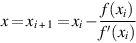
A different approach to division converges to the quotient at a quadratic rather than a linear rate. An actual machine that uses this algorithm will be discussed in Section J.10. First, we will describe the two main iterative algorithms, and then we will discuss the pros and cons of iteration when compared with the direct algorithms. A general technique for constructing iterative algorithms, called Newton’s iteration, is shown in Figure J.13. First, cast the problem in the form of finding the zero of a function. Then, starting from a guess for the zero, approximate the function by its tangent at that guess and form a new guess based on where the tangent has a zero. If xi is a guess at a zero, then the tangent line has the equation:
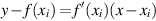

If xi is an estimate for a zero of f, then xi + 1 is a better estimate. To compute xi + 1, find the intersection of the x-axis with the tangent line to f at f(xi).
This equation has a zero at
 J.6.1
J.6.1To recast division as finding the zero of a function, consider f(x) = x− 1 − b. Since the zero of this function is at 1/b, applying Newton’s iteration to it will give an iterative method of computing 1/b from b. Using f ′(x) = − 1/x2, Equation J.6.1 becomes:
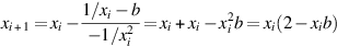 J.6.2
J.6.2
Thus, we could implement computation of a/b using the following method:
Here are some more details. How many times will step 2 have to be iterated? To say that xi is accurate to p bits means that |(xi − 1/b)/(1/b)| = 2− p, and a simple algebraic manipulation shows that when this is so, then (xi + 1 − 1/b)/(1/b) = 2− 2p. Thus, the number of correct bits doubles at each step. Newton’s iteration is self-correcting in the sense that making an error in xi doesn’t really matter. That is, it treats xi as a guess at 1/b and returns xi + 1 as an improvement on it (roughly doubling the digits). One thing that would cause xi to be in error is rounding error. More importantly, however, in the early iterations we can take advantage of the fact that we don’t expect many correct bits by performing the multiplication in reduced precision, thus gaining speed without sacrificing accuracy. Another application of Newton’s iteration is discussed in Exercise J.20.
The second iterative division method is sometimes called Goldschmidt’s algorithm. It is based on the idea that to compute a/b, you should multiply the numerator and denominator by a number r with rb ≈ 1. In more detail, let x0 = a and y0þ = b. At each step compute xi + 1 = rixi and yi + 1 = riyi. Then the quotient xi + 1/yi + 1 = xi/yi = a/b is constant. If we pick ri so that yi → 1, then xi → a/b, so the xi converge to the answer we want. This same idea can be used to compute other functions. For example, to compute the square root of a, let x0 = a and y0 = a, and at each step compute xi + 1 = ri2xi, yi + 1 = riyi. Then xi + 1/yi + 12 = xi/yi2 = 1/a, so if the ri are chosen to drive xi → 1, then  . This technique is used to compute square roots on the TI 8847.
Returning to Goldschmidt’s division algorithm, set x0 = a and y0 = b, and write b = 1 − δ, where |δ| < 1. If we pick r0 = 1 + δ, then y1 = r0y0 = 1 − δ2. We next pick r1 = 1 + δ2, so that y2 = r1y1 = 1 − δ4, and so on. Since |δ| < 1, yi → 1. With this choice of ri, the xi will be computed as 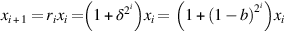 , or
, or
 J.6.3
J.6.3
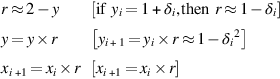
There appear to be two problems with this algorithm. First, convergence is slow when b is not near 1 (that is, δ is not near 0), and, second, the formula isn’t self-correcting—since the quotient is being computed as a product of independent terms, an error in one of them won’t get corrected. To deal with slow convergence, if you want to compute a/b, look up an approximate inverse to b (call it b′), and run the algorithm on ab′/bb′. This will converge rapidly since bb′ ≈ 1.
To deal with the self-correction problem, the computation should be run with a few bits of extra precision to compensate for rounding errors. However, Goldschmidt’s algorithm does have a weak form of self-correction, in that the precise value of the ri does not matter. Thus, in the first few iterations, when the full precision of  is not needed you can choose ri to be a truncation of
  , which may make these iterations run faster without affecting the speed of convergence. If ri is truncated, then yi is no longer exactly . Thus, Equation J.6.3 can no longer be used, but it is easy to organize the computation so that it does not depend on the precise value of ri. With these changes, Goldschmidt’s algorithm is as follows (the notes in brackets show the connection with our earlier formulas).
Loop
End loop
The two iteration methods are related. Suppose in Newton’s method that we unroll the iteration and compute each term xi + 1 directly in terms of b, instead of recursively in terms of xi. By carrying out this calculation (see Exercise J.22), we discover that

This formula is very similar to Equation J.6.3. In fact, they are identical if a and b in J.6.3 are replaced with ax0, bx0, and a = 1. Thus, if the iterations were done to infinite precision, the two methods would yield exactly the same sequence xi.
The advantage of iteration is that it doesn’t require special divide hardware. Instead, it can use the multiplier (which, however, requires extra control). Further, on each step, it delivers twice as many digits as in the previous step—unlike ordinary division, which produces a fixed number of digits at every step.
There are two disadvantages with inverting by iteration. The first is that the IEEE standard requires division to be correctly rounded, but iteration only delivers a result that is close to the correctly rounded answer. In the case of Newton’s iteration, which computes 1/b instead of a/b directly, there is an additional problem. Even if 1/b were correctly rounded, there is no guarantee that a/b will be. An example in decimal with p = 2 is a = 13, b = 51. Then a/b = .2549…, which rounds to .25. But 1/b = .0196…, which rounds to .020, and then a × .020 = .26, which is off by 1. The second disadvantage is that iteration does not give a remainder. This is especially troublesome if the floating-point divide hardware is being used to perform integer division, since a remainder operation is present in almost every high-level language.
Traditional folklore has held that the way to get a correctly rounded result from iteration is to compute 1/b to slightly more than 2p bits, compute a/b to slightly more than 2p bits, and then round to p bits. However, there is a faster way, which apparently was first implemented on the TI 8847. In this method, a/b is computed to about 6 extra bits of precision, giving a preliminary quotient q. By comparing qb with a (again with only 6 extra bits), it is possible to quickly decide whether q is correctly rounded or whether it needs to be bumped up or down by 1 in the least-significant place. This algorithm is explored further in Exercise J.21.
One factor to take into account when deciding on division algorithms is the relative speed of division and multiplication. Since division is more complex than multiplication, it will run more slowly. A common rule of thumb is that division algorithms should try to achieve a speed that is about one-third that of multiplication. One argument in favor of this rule is that there are real programs (such as some versions of spice) where the ratio of division to multiplication is 1:3. Another place where a factor of 3 arises is in the standard iterative method for computing square root. This method involves one division per iteration, but it can be replaced by one using three multiplications. This is discussed in Exercise J.20.
Floating-Point Remainder
For nonnegative integers, integer division and remainder satisfy:

A floating-point remainder x REM y can be similarly defined as x = INT(x/y)y + x REM y. How should x/y be converted to an integer? The IEEE remainder function uses the round-to-even rule. That is, pick n = INT (x/y) so that |x/y − n| ≤ 1/2. If two different n satisfy this relation, pick the even one. Then REM is defined to be x − yn. Unlike integers where 0 ≤ a REM b < b, for floating-point numbers |x REM y| ≤ y/2. Although this defines REM precisely, it is not a practical operational definition, because n can be huge. In single precision, n could be as large as 2127/2− 126 = 2253 ≈ 1076.
There is a natural way to compute REM if a direct division algorithm is used. Proceed as if you were computing x/y. If  and
and  and the divider is as in Figure J.2(b) (page J-4), then load s1 into P and s2 into B. After e1 − e2 division steps, the P register will hold a number r of the form x − yn satisfying 0 ≤ r < y. Since the IEEE remainder satisfies |REM| ≤ y/2, REM is equal to either r or r − y. It is only necessary to keep track of the last quotient bit produced, which is needed to resolve halfway cases. Unfortunately, e1 − e2 can be a lot of steps, and floating-point units typically have a maximum amount of time they are allowed to spend on one instruction. Thus, it is usually not possible to implement REM directly. None of the chips discussed in Section J.10 implements REM, but they could by providing a remainder-step instruction—this is what is done on the Intel 8087 family. A remainder step takes as arguments two numbers x and y, and performs divide steps until either the remainder is in P or n steps have been performed, where n is a small number, such as the number of steps required for division in the highest-supported precision. Then REM can be implemented as a software routine that calls the REM step instruction ⌊(e1 − e2)/n⌋ times, initially using x as the numerator but then replacing it with the remainder from the previous REM step.
REM can be used for computing trigonometric functions. To simplify things, imagine that we are working in base 10 with five significant figures, and consider computing sin x. Suppose that x = 7. Then we can reduce by π = 3.1416 and compute sin(7) = sin(7 − 2 × 3.1416) = sin(0.7168) instead. But, suppose we want to compute sin(2.0 × 10⁵). Then 2 × 10⁵/3.1416 = 63661.8, which in our five-place system comes out to be 63662. Since multiplying 3.1416 times 63662 gives 200000.5392, which rounds to 2.0000 × 10⁵, argument reduction reduces 2 × 10⁵ to 0, which is not even close to being correct. The problem is that our five-place system does not have the precision to do correct argument reduction. Suppose we had the REM operator. Then we could compute 2 × 10⁵ REM 3.1416 and get − .53920. However, this is still not correct because we used 3.1416, which is an approximation for π. The value of 2 × 10⁵ REM π is − .071513.
Traditionally, there have been two approaches to computing periodic functions with large arguments. The first is to return an error for their value when x is large. The second is to store π to a very large number of places and do exact argument reduction. The REM operator is not much help in either of these situations. There is a third approach that has been used in some math libraries, such as the Berkeley UNIX 4.3bsd release. In these libraries, π is computed to the nearest floating-point number. Let’s call this machine π, and denote it by π′. Then, when computing sin x, reduce x using x REM π′. As we saw in the above example, x REM π′ is quite different from x REM π when x is large, so that computing sin x as sin(x REM π′) will not give the exact value of sin x. However, computing trigonometric functions in this fashion has the property that all familiar identities (such as sin2x + cos2x = 1) are true to within a few rounding errors. Thus, using REM together with machine π provides a simple method of computing trigonometric functions that is accurate for small arguments and still may be useful for large arguments.
When REM is used for argument reduction, it is very handy if it also returns the low-order bits of n (where x REM y = x − ny). This is because a practical implementation of trigonometric functions will reduce by something smaller than 2π. For example, it might use π/2, exploiting identities such as sin(x − π/2) = − cos x, sin(x − π) = − sin x. Then the low bits of n are needed to choose the correct identity.
J.7 More on Floating-Point Arithmetic
Before leaving the subject of floating-point arithmetic, we present a few additional topics.
Fused Multiply-Add
Probably the most common use of floating-point units is performing matrix operations, and the most frequent matrix operation is multiplying a matrix times a matrix (or vector), which boils down to computing an inner product, x1 · y1 + x2 · y2 + … + xn · yn. Computing this requires a series of multiply-add combinations.
Motivated by this, the IBM RS/6000 introduced a single instruction that computes ab + c, the fused multiply-add. Although this requires being able to read three operands in a single instruction, it has the potential for improving the performance of computing inner products.
The fused multiply-add computes ab + c exactly and then rounds. Although rounding only once increases the accuracy of inner products somewhat, that is not its primary motivation. There are two main advantages of rounding once. First, as we saw in the previous sections, rounding is expensive to implement because it may require an addition. By rounding only once, an addition operation has been eliminated. Second, the extra accuracy of fused multiply-add can be used to compute correctly rounded division and square root when these are not available directly in hardware. Fused multiply-add can also be used to implement efficient floating-point multiple-precision packages.
The implementation of correctly rounded division using fused multiply-add has many details, but the main idea is simple. Consider again the example from Section J.6 (page J-30), which was computing a/b with a = 13, b = 51. Then 1/b rounds to b′ = .020, and ab′ rounds to q′ = .26, which is not the correctly rounded quotient. Applying fused multiply-add twice will correctly adjust the result, via the formulas

Computing to two-digit accuracy, bq′ = 51 × .26 rounds to 13, and so r = a − bq′ would be 0, giving no adjustment. But using fused multiply-add gives r = a − bq′ = 13 − (51 × .26) = − .26, and then q″ = q′ + rb′ = .26 − .0052 = .2548, which rounds to the correct quotient, .25. More details can be found in the papers by Montoye, Hokenek, and Runyon [1990] and Markstein [1990].
Precisions
The standard specifies four precisions: single, single extended, double, and double extended. The properties of these precisions are summarized in Figure J.7 (page J-16). Implementations are not required to have all four precisions, but are encouraged to support either the combination of single and single extended or all of single, double, and double extended. Because of the widespread use of double precision in scientific computing, double precision is almost always implemented. Thus, the computer designer usually only has to decide whether to support double extended and, if so, how many bits it should have.
The Motorola 68882 and Intel 387 coprocessors implement extended precision using the smallest allowable size of 80 bits (64 bits of significand). However, many of the more recently designed, high-performance floating-point chips do not implement 80-bit extended precision. One reason is that the 80-bit width of extended precision is awkward for 64-bit buses and registers. Some new architectures, such as SPARC V8 and PA-RISC, specify a 128-bit extended (or quad) precision. They have established a de facto convention for quad that has 15 bits of exponent and 113 bits of significand.
Although most high-level languages do not provide access to extended precision, it is very useful to writers of mathematical software. As an example, consider writing a library routine to compute the length of a vector (x,y) in the plane, namely,  . If x is larger than
  , then computing this in the obvious way will overflow. This means that either the allowable exponent range for this subroutine will be cut in half or a more complex algorithm using scaling will have to be employed. But, if extended precision is available, then the simple algorithm will work. Computing the length of a vector is a simple task, and it is not difficult to come up with an algorithm that doesn’t overflow. However, there are more complex problems for which extended precision means the difference between a simple, fast algorithm and a much more complex one. One of the best examples of this is binary-to-decimal conversion. An efficient algorithm for binary-to-decimal conversion that makes essential use of extended precision is very readably presented in Coonen [1984]. This algorithm is also briefly sketched in Goldberg [1991]. Computing accurate values for transcendental functions is another example of a problem that is made much easier if extended precision is present.
One very important fact about precision concerns double rounding. To illustrate in decimals, suppose that we want to compute 1.9 × 0.66 and that single precision is two digits, while extended precision is three digits. The exact result of the product is 1.254. Rounded to extended precision, the result is 1.25. When further rounded to single precision, we get 1.2. However, the result of 1.9 × 0.66 correctly rounded to single precision is 1.3. Thus, rounding twice may not produce the same result as rounding once. Suppose you want to build hardware that only does double-precision arithmetic. Can you simulate single precision by computing first in double precision and then rounding to single? The above example suggests that you can’t. However, double rounding is not always dangerous. In fact, the following rule is true (this is not easy to prove, but see Exercise J.25).
If x and y have p-bit significands, and x + y is computed exactly and then rounded to q places, a second rounding to p places will not change the answer if q ≥ 2p + 2. This is true not only for addition, but also for multiplication, division, and square root.
In our example above, q = 3 and p = 2, so q Š 2p + 2 is not true. On the other hand, for IEEE arithmetic, double precision has q = 53 and p = 24, so q = 53 Š 2p + 2 = 50. Thus, single precision can be implemented by computing in double precision—that is, computing the answer exactly and then rounding to double—and then rounding to single precision.
Exceptions
The IEEE standard defines five exceptions: underflow, overflow, divide by zero, inexact, and invalid. By default, when these exceptions occur, they merely set a flag and the computation continues. The flags are sticky, meaning that once set they remain set until explicitly cleared. The standard strongly encourages implementations to provide a trap-enable bit for each exception. When an exception with an enabled trap handler occurs, a user trap handler is called, and the value of the associated exception flag is undefined. In Section J.3 we mentioned that  has the value NaN and 1/0 is ∞. These are examples of operations that raise an exception. By default, computing sets the invalid flag and returns the value NaN. Similarly 1/0 sets the divide-by-zero flag and returns ∞.
The underflow, overflow, and divide-by-zero exceptions are found in most other systems. The invalid exception is for the result of operations such as , 0/0, or ∞ − ∞, which don’t have any natural value as a floating-point number or as ± ∞. The inexact exception is peculiar to IEEE arithmetic and occurs either when the result of an operation must be rounded or when it overflows. In fact, since 1/0 and an operation that overflows both deliver ∞, the exception flags must be consulted to distinguish between them. The inexact exception is an unusual “exception,” in that it is not really an exceptional condition because it occurs so frequently. Thus, enabling a trap handler for the inexact exception will most likely have a severe impact on performance. Enabling a trap handler doesn’t affect whether an operation is exceptional except in the case of underflow. This is discussed below.
The IEEE standard assumes that when a trap occurs, it is possible to identify the operation that trapped and its operands. On machines with pipelining or multiple arithmetic units, when an exception occurs, it may not be enough to simply have the trap handler examine the program counter. Hardware support may be necessary to identify exactly which operation trapped.
Another problem is illustrated by the following program fragment.
r1 = r2/r3
r2 = r4 + r5
These two instructions might well be executed in parallel. If the divide traps, its argument r2 could already have been overwritten by the addition, especially since addition is almost always faster than division. Computer systems that support trapping in the IEEE standard must provide some way to save the value of r2, either in hardware or by having the compiler avoid such a situation in the first place. This kind of problem is not peculiar to floating point. In the sequence
r1 = 0(r2)
r2 = r3
it would be efficient to execute r2 = r3 while waiting for memory. But, if accessing 0(r2) causes a page fault, r2 might no longer be available for restarting the instruction r1 = 0(r2).
One approach to this problem, used in the MIPS R3010, is to identify instructions that may cause an exception early in the instruction cycle. For example, an addition can overflow only if one of the operands has an exponent of Emax, and so on. This early check is conservative: It might flag an operation that doesn’t actually cause an exception. However, if such false positives are rare, then this technique will have excellent performance. When an instruction is tagged as being possibly exceptional, special code in a trap handler can compute it without destroying any state. Remember that all these problems occur only when trap handlers are enabled. Otherwise, setting the exception flags during normal processing is straightforward.
Underflow
We have alluded several times to the fact that detection of underflow is more complex than for the other exceptions. The IEEE standard specifies that if an underflow trap handler is enabled, the system must trap if the result is denormal. On the other hand, if trap handlers are disabled, then the underflow flag is set only if there is a loss of accuracy—that is, if the result must be rounded. The rationale is, if no accuracy is lost on an underflow, there is no point in setting a warning flag. But if a trap handler is enabled, the user might be trying to simulate flush-to-zero and should therefore be notified whenever a result dips below .
So if there is no trap handler, the underflow exception is signaled only when the result is denormal and inexact, but the definitions of denormal and inexact are both subject to multiple interpretations. Normally, inexact means there was a result that couldn’t be represented exactly and had to be rounded. Consider the example (in a base 2 floating-point system with 3-bit significands) of  , with round to nearest in effect. The delivered result is
  , which had to be rounded, causing inexact to be signaled. But is it correct to also signal underflow? Gradual underflow loses significance because the exponent range is bounded. If the exponent range were unbounded, the delivered result would be
  , exactly the same answer obtained with gradual underflow. The fact that denormalized numbers have fewer bits in their significand than normalized numbers therefore doesn’t make any difference in this case. The commentary to the standard [Cody et al. 1984] encourages this as the criterion for setting the underflow flag. That is, it should be set whenever the delivered result is different from what would be delivered in a system with the same fraction size, but with a very large exponent range. However, owing to the difficulty of implementing this scheme, the standard allows setting the underflow flag whenever the result is denormal and different from the infinitely precise result.
There are two possible definitions of what it means for a result to be denormal. Consider the example of 1.102 × 2− 1 multiplied by  . The exact product is
  . The rounded result is the normal number
  . Should underflow be signaled? Signaling underflow means that you are using the before rounding rule, because the result was denormal before rounding. Not signaling underflow means that you are using the after rounding rule, because the result is normalized after rounding. The IEEE standard provides for choosing either rule; however, the one chosen must be used consistently for all operations.
To illustrate these rules, consider floating-point addition. When the result of an addition (or subtraction) is denormal, it is always exact. Thus, the underflow flag never needs to be set for addition. That’s because if traps are not enabled then no exception is raised. And if traps are enabled, the value of the underflow flag is undefined, so again it doesn’t need to be set.
One final subtlety should be mentioned concerning underflow. When there is no underflow trap handler, the result of an operation on p-bit numbers that causes an underflow is a denormal number with p − 1 or fewer bits of precision. When traps are enabled, the trap handler is provided with the result of the operation rounded to p bits and with the exponent wrapped around. Now there is a potential double-rounding problem. If the trap handler wants to return the denormal result, it can’t just round its argument, because that might lead to a double-rounding error. Thus, the trap handler must be passed at least one extra bit of information if it is to be able to deliver the correctly rounded result.
J.8 Speeding Up Integer Addition
The previous section showed that many steps go into implementing floating-point operations; however, each floating-point operation eventually reduces to an integer operation. Thus, increasing the speed of integer operations will also lead to faster floating point.
Integer addition is the simplest operation and the most important. Even for programs that don’t do explicit arithmetic, addition must be performed to increment the program counter and to calculate addresses. Despite the simplicity of addition, there isn’t a single best way to perform high-speed addition. We will discuss three techniques that are in current use: carry-lookahead, carry-skip, and carry-select.
Carry-Lookahead
An n-bit adder is just a combinational circuit. It can therefore be written by a logic formula whose form is a sum of products and can be computed by a circuit with two levels of logic. How do you figure out what this circuit looks like? From Equation J.2.1 (page J-3) the formula for the ith sum can be written as:
 J.8.1
J.8.1
where ci is both the carry-in to the ith adder and the carry-out from the (i − 1)-st adder.
The problem with this formula is that, although we know the values of ai and bi—they are inputs to the circuit—we don’t know ci. So our goal is to write ci in terms of ai and bi. To accomplish this, we first rewrite Equation J.2.2 (page J-3) as:
 J.8.2
J.8.2
Here is the reason for the symbols p and g: If gi − 1 is true, then ci is certainly true, so a carry is generated. Thus, g is for generate. If pi − 1 is true, then if ci − 1 is true, it is propagated to ci. Start with Equation J.8.1 and use Equation J.8.2 to replace ci with gi − 1 + pi − 1ci − 1. Then, use Equation J.8.2 with i − 1 in place of i to replace ci − 1 with ci − 2, and so on. This gives the result: