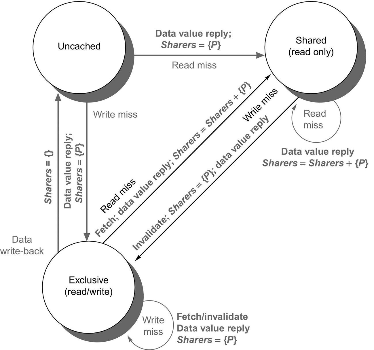
All actions are in gray because they are all externally caused. Bold indicates the action taken by the directory in response to the request.
To understand these directory operations, let's examine the requests received and actions taken state by state. When a block is in the uncached state, the copy in memory is the current value, so the only possible requests for that block are
 Read miss—The requesting node is sent the requested data from memory, and the requester is made the only sharing node. The state of the block is made shared.
- Write miss—The requesting node is sent the value and becomes the sharing node. The block is made exclusive to indicate that the only valid copy is cached. Sharers indicates the identity of the owner.
When the block is in the shared state, the memory value is up to date, so the same two requests can occur:
- Read miss—The requesting node is sent the requested data from memory, and the requesting node is added to the sharing set.
- Write miss—The requesting node is sent the value. All nodes in the set Sharers are sent invalidate messages, and the Sharers set is to contain the identity of the requesting node. The state of the block is made exclusive.
When the block is in the exclusive state, the current value of the block is held in a cache on the node identified by the set Sharers (the owner), so there are three possible directory requests:
- Read miss—The owner is sent a data fetch message, which causes the state of the block in the owner's cache to transition to shared and causes the owner to send the data to the directory, where it is written to memory and sent back to the requesting processor. The identity of the requesting node is added to the set Sharers, which still contains the identity of the processor that was the owner (since it still has a readable copy).
- Data write-back—The owner is replacing the block and therefore must write it back. This write-back makes the memory copy up to date (the home directory essentially becomes the owner), the block is now uncached, and the Sharers set is empty.
- Write miss—The block has a new owner. A message is sent to the old owner, causing the cache to invalidate the block and send the value to the directory, from which it is sent to the requesting node, which becomes the new owner. Sharers is set to the identity of the new owner, and the state of the block remains exclusive.
This state transition diagram in Figure 5.21 is a simplification, just as it was in the snooping cache case. In the case of a directory, as well as a snooping scheme implemented with a network other than a bus, our protocols will need to deal with nonatomic memory transactions. Appendix I explores these issues in depth.
The directory protocols used in real multiprocessors contain additional optimizations. In particular, in this protocol when a read or write miss occurs for a block that is exclusive, the block is first sent to the directory at the home node. From there it is stored into the home memory and also sent to the original requesting node. Many of the protocols in use in commercial multiprocessors forward the data from the owner node to the requesting node directly (as well as performing the write-back to the home). Such optimizations often add complexity by increasing the possibility of deadlock and by increasing the types of messages that must be handled.
Implementing a directory scheme requires solving most of the same challenges we discussed for snooping protocols. There are, however, new and additional problems, which we describe in Appendix I. In Section 5.8, we briefly describe how modern multicores extend coherence beyond a single chip. The combinations of multichip coherence and multicore coherence include all four possibilities of snooping/snooping (AMD Opteron), snooping/directory, directory/snooping, and directory/directory! Many multiprocessors have chosen some form of snooping within a single chip, which is attractive if the outermost cache is shared and inclusive, and directories across multiple chips. Such an approach simplifies implementation because only the processor chip, rather than an individual core, need be tracked.
5.5 Synchronization: The Basics
Synchronization mechanisms are typically built with user-level software routines that rely on hardware-supplied synchronization instructions. For smaller multiprocessors or low-contention situations, the key hardware capability is an uninterruptible instruction or instruction sequence capable of atomically retrieving and changing a value. Software synchronization mechanisms are then constructed using this capability. In this section, we focus on the implementation of lock and unlock synchronization operations. Lock and unlock can be used straightforwardly to create mutual exclusion, as well as to implement more complex synchronization mechanisms.
In high-contention situations, synchronization can become a performance bottleneck because contention introduces additional delays and because latency is potentially greater in such a multiprocessor. We discuss how the basic synchronization mechanisms of this section can be extended for large processor counts in Appendix I.
Basic Hardware Primitives
The key ability we require to implement synchronization in a multiprocessor is a set of hardware primitives with the ability to atomically read and modify a memory location. Without such a capability, the cost of building basic synchronization primitives will be too high and will increase as the processor count increases. There are a number of alternative formulations of the basic hardware primitives, all of which provide the ability to atomically read and modify a location, together with some way to tell whether the read and write were performed atomically. These hardware primitives are the basic building blocks that are used to build a wide variety of user-level synchronization operations, including things such as locks and barriers. In general, architects do not expect users to employ the basic hardware primitives, but instead expect that the primitives will be used by system programmers to build a synchronization library, a process that is often complex and tricky. Let's start with one such hardware primitive and show how it can be used to build some basic synchronization operations.
One typical operation for building synchronization operations is the atomic exchange, which interchanges a value in a register for a value in memory. To see how to use this to build a basic synchronization operation, assume that we want to build a simple lock where the value 0 is used to indicate that the lock is free and 1 is used to indicate that the lock is unavailable. A processor tries to set the lock by doing an exchange of 1, which is in a register, with the memory address corresponding to the lock. The value returned from the exchange instruction is 1 if some other processor had otherwise already claimed access and 0. In the latter case, the value is also changed to 1, preventing any competing exchange from also retrieving a 0.
For example, consider two processors that each try to do the exchange simultaneously: This race is broken because exactly one of the processors will perform the exchange first, returning 0, and the second processor will return 1 when it does the exchange. The key to using the exchange (or swap) primitive to implement synchronization is that the operation is atomic: the exchange is indivisible, and two simultaneous exchanges will be ordered by the write serialization mechanisms. It is impossible for two processors trying to set the synchronization variable in this manner to both determine they have simultaneously set the variable.
There are a number of other atomic primitives that can be used to implement synchronization. They all have the key property that they read and update a memory value in such a manner that we can tell whether the two operations executed atomically. One operation, present in many older multiprocessors, is test-and-set, which tests a value and sets it if the value passes the test. For example, we could define an operation that tested for 0 and set the value to 1, which can be used in a fashion similar to how we used atomic exchange. Another atomic synchronization primitive is fetch-and-increment: it returns the value of a memory location and atomically increments it. By using the value 0 to indicate that the synchronization variable is unclaimed, we can use fetch-and-increment, just as we used exchange. There are other uses of operations like fetch-and-increment, which we will see shortly.
Implementing a single atomic memory operation introduces some challenges because it requires both a memory read and a write in a single, uninterruptible instruction. This requirement complicates the implementation of coherence because the hardware cannot allow any other operations between the read and the write, and yet must not deadlock.
An alternative is to have a pair of instructions where the second instruction returns a value from which it can be deduced whether the pair of instructions was executed as though the instructions were atomic. The pair of instructions is effectively atomic if it appears as though all other operations executed by any processor occurred before or after the pair. Thus, when an instruction pair is effectively atomic, no other processor can change the value between the instruction pair. This is the approach used in the MIPS processors and in RISC V.
In RISC V, the pair of instructions includes a special load called a load reserved (also called load linked or load locked) and a special store called a store conditional. Load reserved loads the contents of memory given by rs1 into rd and creates a reservation on that memory address. Store conditional stores the value in rs2 into the memory address given by rs1. If the reservation of the load is broken by a write to the same memory location, the store conditional fails and writes a nonzero to rd; if it succeeds, the store conditional writes 0. If the processor does a context switch between the two instructions, then the store conditional always fails.
These instructions are used in sequence, and because the load reserved returns the initial value and the store conditional returns 0 only if it succeeds, the following sequence implements an atomic exchange on the memory location specified by the contents of x1 with the value in x4:
try:     mov    x3,x4   ;mov exchange value
          lr    x2,x1   ;load reserved from
          sc    x3,0(x1);store conditional
         bnez   x3,try  ;branch store fails
         mov    x4,x2   ;put load value in x4
At the end of this sequence, the contents of x4 and the memory location specified by x1 have been atomically exchanged. Anytime a processor intervenes and modifies the value in memory between the lr and sc instructions, the sc returns 0 in x3, causing the code sequence to try again.
An advantage of the load reserved/store conditional mechanism is that it can be used to build other synchronization primitives. For example, here is an atomic fetch-and-increment:
try:      lr    x2,x1    ;load reserved 0(x1)
          addi  x3,x2,1  ;increment
          sc    x3,0(x1) ;store conditional
          bnez  x3,try   ;branch store fails
These instructions are typically implemented by keeping track of the address specified in the lr instruction in a register, often called the reserved register. If an interrupt occurs, or if the cache block matching the address in the link register is invalidated (e.g., by another sc), the link register is cleared. The sc instruction simply checks that its address matches that in the reserved register. If so, the sc succeeds; otherwise, it fails. Because the store conditional will fail after either another attempted store to the load reserved address or any exception, care must be taken in choosing what instructions are inserted between the two instructions. In particular, only register-register instructions can safely be permitted; otherwise, it is possible to create deadlock situations where the processor can never complete the sc. In addition, the number of instructions between the load reserved and the store conditional should be small to minimize the probability that either an unrelated event or a competing processor causes the store conditional to fail frequently.
Implementing Locks Using Coherence
Once we have an atomic operation, we can use the coherence mechanisms of a multiprocessor to implement spin locks—locks that a processor continuously tries to acquire, spinning around a loop until it succeeds. Spin locks are used when programmers expect the lock to be held for a very short amount of time and when they want the process of locking to be low latency when the lock is available. Because spin locks tie up the processor waiting in a loop for the lock to become free, they are inappropriate in some circumstances.
The simplest implementation, which we would use if there were no cache coherence, would be to keep the lock variables in memory. A processor could continually try to acquire the lock using an atomic operation, say, atomic exchange, and test whether the exchange returned the lock as free. To release the lock, the processor simply stores the value 0 to the lock. Here is the code sequence to lock a spin lock whose address is in x1. It uses EXCH as a macro for the atomic exchange sequence from page 414:
          addi x2,R0,#1
lockit:   EXCH x2,0(x1)    ;atomic exchange
          bnez x2,lockit   ;already locked?
If our multiprocessor supports cache coherence, we can cache the locks using the coherence mechanism to maintain the lock value coherently. Caching locks has two advantages. First, it allows an implementation where the process of “spinning” (trying to test and acquire the lock in a tight loop) could be done on a local cached copy rather than requiring a global memory access on each attempt to acquire the lock. The second advantage comes from the observation that there is often locality in lock accesses; that is, the processor that used the lock last will use it again in the near future. In such cases, the lock value may reside in the cache of that processor, greatly reducing the time to acquire the lock.
Obtaining the first advantage—being able to spin on a local cached copy rather than generating a memory request for each attempt to acquire the lock—requires a change in our simple spin procedure. Each attempt to exchange in the preceding loop requires a write operation. If multiple processors are attempting to get the lock, each will generate the write. Most of these writes will lead to write misses because each processor is trying to obtain the lock variable in an exclusive state.
Thus we should modify our spin lock procedure so that it spins by doing reads on a local copy of the lock until it successfully sees that the lock is available. Then it attempts to acquire the lock by doing a swap operation. A processor first reads the lock variable to test its state. A processor keeps reading and testing until the value of the read indicates that the lock is unlocked. The processor then races against all other processes that were similarly “spin waiting” to see which can lock the variable first. All processes use a swap instruction that reads the old value and stores a 1 into the lock variable. The single winner will see the 0, and the losers will see a 1 that was placed there by the winner. (The losers will continue to set the variable to the locked value, but that doesn't matter.) The winning processor executes the code after the lock and, when finished, stores a 0 into the lock variable to release the lock, which starts the race all over again. Here is the code to perform this spin lock (remember that 0 is unlocked and 1 is locked):
lockit:   ld   x2,0(x1)  ;load of lock
          bnez x2,lockit ;not available-spin
          addi x2,R0,#1  ;load locked value
          EXCH x2,0(x1)  ;swap
          bnez x2,lockit ;branch if lock wasn’t 0
Let's examine how this “spin lock” scheme uses the cache coherence mechanisms. Figure 5.22 shows the processor and bus or directory operations for multiple processes trying to lock a variable using an atomic swap. Once the processor with the lock stores a 0 into the lock, all other caches are invalidated and must fetch the new value to update their copy of the lock. One such cache gets the copy of the unlocked value (0) first and performs the swap. When the cache miss of other processors is satisfied, they find that the variable is already locked, so they must return to testing and spinning.
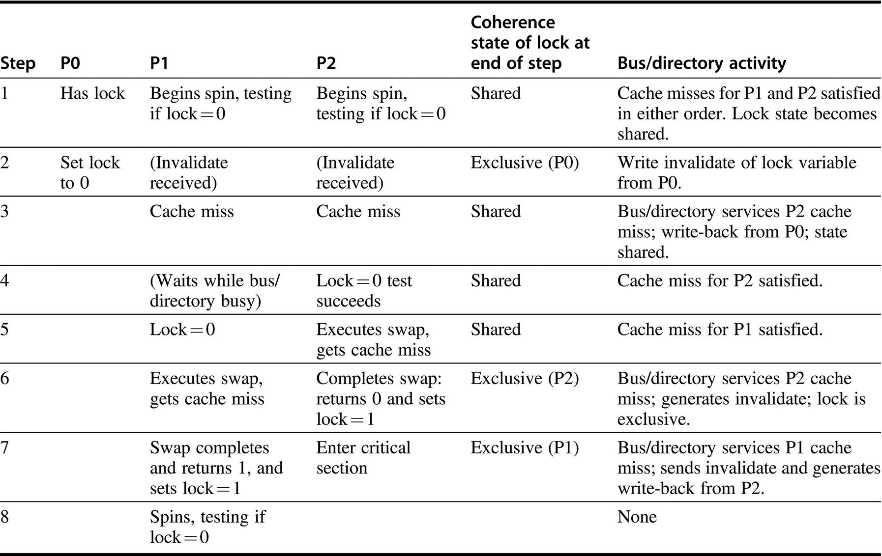
P0 exits and unlocks the lock (step 2). P1 and P2 race to see which reads the unlocked value during the swap (steps 3–5). P2 wins and enters the critical section (steps 6 and 7), while P1's attempt fails, so it starts spin waiting (steps 7 and 8). In a real system, these events will take many more than 8 clock ticks because acquiring the bus and replying to misses take much longer. Once step 8 is reached, the process can repeat with P2, eventually getting exclusive access and setting the lock to 0.
This example shows another advantage of the load reserved/store conditional primitives: the read and write operations are explicitly separated. The load reserved need not cause any bus traffic. This fact allows the following simple code sequence, which has the same characteristics as the optimized version using exchange (x1 has the address of the lock, the lr has replaced the LD, and the sc has replaced the EXCH):
lockit:   lr   x2,0(x1)   ;load reserved
          bnez x2,lockit  ;not available-spin
          addi x2,R0,#1   ;locked value
          sc   x2,0(x1)   ;store
          bnez x2,lockit  ;branch if store fails
The first branch forms the spinning loop; the second branch resolves races when two processors see the lock available simultaneously.
5.6 Models of Memory Consistency: An Introduction
Cache coherence ensures that multiple processors see a consistent view of memory. It does not answer the question of how consistent the view of memory must be. By “how consistent,” we are really asking when a processor must see a value that has been updated by another processor. Because processors communicate through shared variables (used both for data values and for synchronization), the question boils down to this: In what order must a processor observe the data writes of another processor? Because the only way to “observe the writes of another processor” is through reads, the question becomes what properties must be enforced among reads and writes to different locations by different processors?
Although the question of how consistent memory must be seems simple, it is remarkably complicated, as we can see with a simple example. Here are two code segments from processes P1 and P2, shown side by side:
 P1:         A = 0;          P2:    B = 0;
             .....                 .....
             A = 1;                 B = 1;
 L1:         if (B == 0)…    L2:   if (A == 0)…
Assume that the processes are running on different processors, and that locations A and B are originally cached by both processors with the initial value of 0. If writes always take immediate effect and are immediately seen by other processors, it will be impossible for both IF statements (labeled L1 and L2) to evaluate their conditions as true, since reaching the IF statement means that either A or B must have been assigned the value 1. But suppose the write invalidate is delayed, and the processor is allowed to continue during this delay. Then it is possible that both P1 and P2 have not seen the invalidations for B and A (respectively) before they attempt to read the values. The question now is should this behavior be allowed, and, if so, under what conditions?
The most straightforward model for memory consistency is called sequential consistency. Sequential consistency requires that the result of any execution be the same as though the memory accesses executed by each processor were kept in order and the accesses among different processors were arbitrarily interleaved. Sequential consistency eliminates the possibility of some nonobvious execution in the previous example because the assignments must be completed before the IF statements are initiated.
The simplest way to implement sequential consistency is to require a processor to delay the completion of any memory access until all the invalidations caused by that access are completed. Of course, it is equally effective to delay the next memory access until the previous one is completed. Remember that memory consistency involves operations among different variables: the two accesses that must be ordered are actually to different memory locations. In our example, we must delay the read of A or B (A == 0 or B == 0) until the previous write has completed (B = 1 or A = 1). Under sequential consistency, we cannot, for example, simply place the write in a write buffer and continue with the read.
Although sequential consistency presents a simple programming paradigm, it reduces potential performance, especially in a multiprocessor with a large number of processors or long interconnect delays, as we can see in the following example.
To provide better performance, researchers and architects have explored two different routes. First, they developed ambitious implementations that preserve sequential consistency but use latency-hiding techniques to reduce the penalty; we discuss these in Section 5.7. Second, they developed less restrictive memory consistency models that allow for faster hardware. Such models can affect how the programmer sees the multiprocessor, so before we discuss these less restrictive models, let's look at what the programmer expects.
The Programmer's View
Although the sequential consistency model has a performance disadvantage, from the viewpoint of the programmer, it has the advantage of simplicity. The challenge is to develop a programming model that is simple to explain and yet allows a high-performance implementation.
One such programming model that allows us to have a more efficient implementation is to assume that programs are synchronized. A program is synchronized if all accesses to shared data are ordered by synchronization operations. A data reference is ordered by a synchronization operation if, in every possible execution, a write of a variable by one processor and an access (either a read or a write) of that variable by another processor are separated by a pair of synchronization operations, one executed after the write by the writing processor and one executed before the access by the second processor. Cases where variables may be updated without ordering by synchronization are called data races because the execution outcome depends on the relative speed of the processors, and like races in hardware design, the outcome is unpredictable, which leads to another name for synchronized programs: data-race-free.
As a simple example, consider a variable being read and updated by two different processors. Each processor surrounds the read and update with a lock and an unlock, both to ensure mutual exclusion for the update and to ensure that the read is consistent. Clearly, every write is now separated from a read by the other processor by a pair of synchronization operations: one unlock (after the write) and one lock (before the read). Of course, if two processors are writing a variable with no intervening reads, then the writes must also be separated by synchronization operations.
It is a broadly accepted observation that most programs are synchronized. This observation is true primarily because, if the accesses were unsynchronized, the behavior of the program would likely be unpredictable because the speed of execution would determine which processor won a data race and thus affect the results of the program. Even with sequential consistency, reasoning about such programs is very difficult.
Programmers could attempt to guarantee ordering by constructing their own synchronization mechanisms, but this is extremely tricky, can lead to buggy programs, and may not be supported architecturally, meaning that they may not work in future generations of the multiprocessor. Instead, almost all programmers will choose to use synchronization libraries that are correct and optimized for the multiprocessor and the type of synchronization.
Finally, the use of standard synchronization primitives ensures that even if the architecture implements a more relaxed consistency model than sequential consistency, a synchronized program will behave as though the hardware implemented sequential consistency.
Relaxed Consistency Models: The Basics and Release Consistency
The key idea in relaxed consistency models is to allow reads and writes to complete out of order, but to use synchronization operations to enforce ordering so that a synchronized program behaves as though the processor were sequentially consistent. There are a variety of relaxed models that are classified according to what read and write orderings they relax. We specify the orderings by a set of rules of the form X → Y, meaning that operation X must complete before operation Y is done. Sequential consistency requires maintaining all four possible orderings: R → W, R → R, W → R, and W → W. The relaxed models are defined by the subset of four orderings they relax:
- 1. Relaxing only the W → R ordering yields a model known as total store ordering or processor consistency. Because this model retains ordering among writes, many programs that operate under sequential consistency operate under this model, without additional synchronization.
- 2. Relaxing both the W → R ordering and the W → W ordering yields a model known as partial store order.
- 3. Relaxing all four orderings yields a variety of models including weak ordering, the PowerPC consistency model, and release consistency, the RISC V consistency model.
By relaxing these orderings, the processor may obtain significant performance advantages, which is the reason that RISC V, ARMv8, as well as the C++ and C language standards chose release consistency as the model.
Release consistency distinguishes between synchronization operations that are used to acquire access to a shared variable (denoted SA) and those that release an object to allow another processor to acquire access (denoted SR). Release consistency is based on the observation that in synchronized programs, an acquire operation must precede a use of shared data, and a release operation must follow any updates to shared data and also precede the time of the next acquire. This property allows us to slightly relax the ordering by observing that a read or write that precedes an acquire need not complete before the acquire, and also that a read or write that follows a release need not wait for the release. Thus the orderings that are preserved involve only SA and SR, as shown in Figure 5.23; as the example in Figure 5.24 shows, this model imposes the fewest orders of the five models.
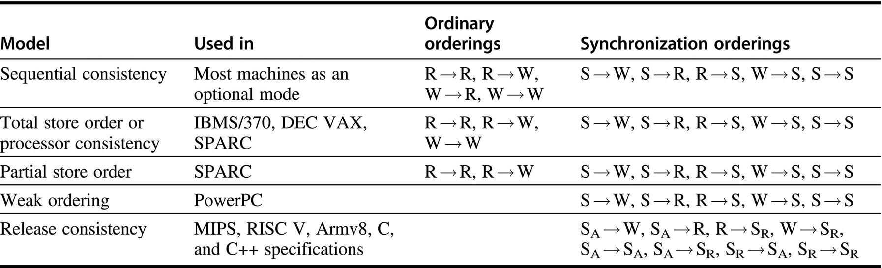
The models grow from most restrictive (sequential consistency) to least restrictive (release consistency), allowing increased flexibility in the implementation. The weaker models rely on fences created by synchronization operations, as opposed to an implicit fence at every memory operation. SA and SR stand for acquire and release operations, respectively, and are needed to define release consistency. If we were to use the notation SA and SR for each S consistently, each ordering with one S would become two orderings (e.g., S → W becomes SA → W, SR → W), and each S → S would become the four orderings shown in the last line of the bottom-right table entry.
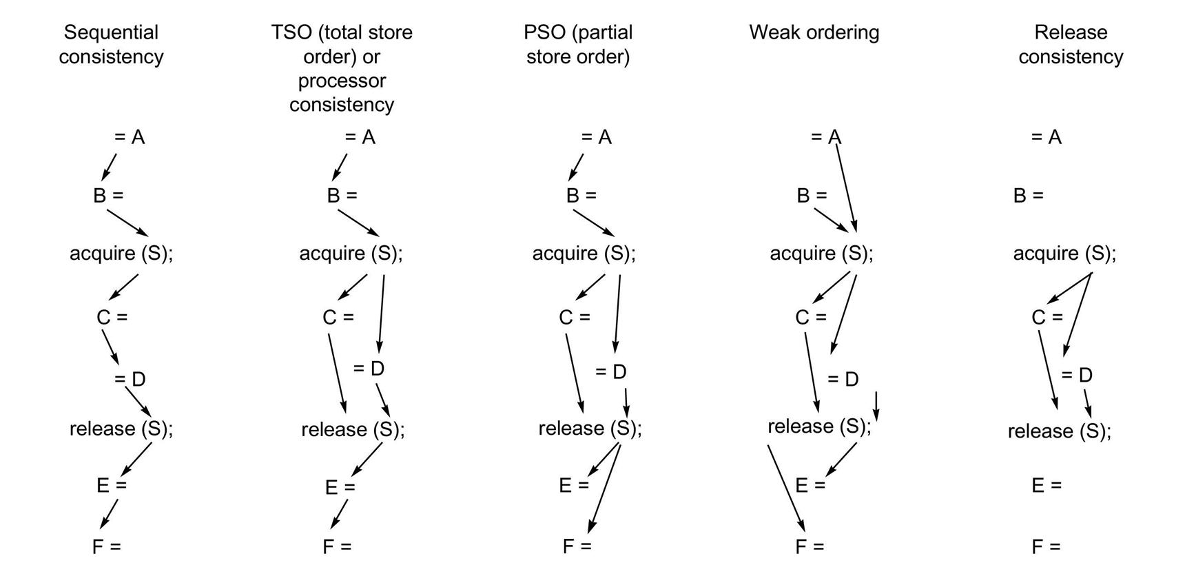
Only the minimum orders are shown with arrows. Orders implied by transitivity, such as the write of C before the release of S in the sequential consistency model or the acquire before the release in weak ordering or release consistency, are not shown.
Release consistency provides one of the least restrictive models that is easily checkable and ensures that synchronized programs will see a sequentially consistent execution. Although most synchronization operations are either an acquire or a release (an acquire normally reads a synchronization variable and atomically updates it, and a release usually just writes it), some operations, such as a barrier, act as both an acquire and a release and cause the ordering to be equivalent to weak ordering. Although synchronization operations always ensure that previous writes have completed, we may want to guarantee that writes are completed without an identified synchronization operation. In such cases, an explicit instruction, called FENCE in RISC V, is used to ensure that all previous instructions in that thread have completed, including completion of all memory writes and associated invalidates. For more information about the complexities, implementation issues, and performance potential from relaxed models, we highly recommend the excellent tutorial by Adve and Gharachorloo (1996).
5.7 Cross-Cutting Issues
Because multiprocessors redefine many system characteristics (e.g., performance assessment, memory latency, and the importance of scalability), they introduce interesting design problems that cut across the spectrum, affecting both hardware and software. In this section, we give several examples related to the issue of memory consistency. We then examine the performance gained when multithreading is added to multiprocessing.
Compiler Optimization and the Consistency Model
Another reason for defining a model for memory consistency is to specify the range of legal compiler optimizations that can be performed on shared data. In explicitly parallel programs, unless the synchronization points are clearly defined and the programs are synchronized, the compiler cannot interchange a read and a write of two different shared data items because such transformations might affect the semantics of the program. This restriction prevents even relatively simple optimizations, such as register allocation of shared data, because such a process usually interchanges reads and writes. In implicitly parallelized programs—for example, those written in High Performance Fortran (HPF)—programs must be synchronized and the synchronization points are known, so this issue does not arise. Whether compilers can get significant advantage from more relaxed consistency models remains an open question, both from a research viewpoint and from a practical viewpoint, where the lack of uniform models is likely to retard progress on deploying compilers.
Using Speculation to Hide Latency in Strict Consistency Models
As we saw in Chapter 3, speculation can be used to hide memory latency. It can also be used to hide latency arising from a strict consistency model, giving much of the benefit of a relaxed memory model. The key idea is for the processor to use dynamic scheduling to reorder memory references, letting them possibly execute out of order. Executing the memory references out of order may generate violations of sequential consistency, which might affect the execution of the program. This possibility is avoided by using the delayed commit feature of a speculative processor. Assume the coherency protocol is based on invalidation. If the processor receives an invalidation for a memory reference before the memory reference is committed, the processor uses speculation recovery to back out of the computation and restart with the memory reference whose address was invalidated.
If the reordering of memory requests by the processor yields an execution order that could result in an outcome that differs from what would have been seen under sequential consistency, the processor will redo the execution. The key to using this approach is that the processor need only guarantee that the result would be the same as if all accesses were completed in order, and it can achieve this by detecting when the results might differ. The approach is attractive because the speculative restart will rarely be triggered. It will be triggered only when there are unsynchronized accesses that actually cause a race (Gharachorloo et al., 1992).
Hill (1998) advocated the combination of sequential or processor consistency together with speculative execution as the consistency model of choice. His argument has three parts. First, an aggressive implementation of either sequential consistency or processor consistency will gain most of the advantage of a more relaxed model. Second, such an implementation adds very little to the implementation cost of a speculative processor. Third, such an approach allows the programmer to reason using the simpler programming models of either sequential or processor consistency. The MIPS R10000 design team had this insight in the mid-1990s and used the R10000's out-of-order capability to support this type of aggressive implementation of sequential consistency.
One open question is how successful compiler technology will be in optimizing memory references to shared variables. The state of optimization technology and the fact that shared data are often accessed via pointers or array indexing have limited the use of such optimizations. If this technology were to become available and lead to significant performance advantages, compiler writers would want to be able to take advantage of a more relaxed programming model. This possibility and the desire to keep the future as flexible as possible led the RISC V designers to opt for release consistency, after a long series of debates.
Inclusion and Its Implementation
All multiprocessors use multilevel cache hierarchies to reduce both the demand on the global interconnect and the latency of cache misses. If the cache also provides multilevel inclusion—every level of cache hierarchy is a subset of the level farther away from the processor—then we can use the multilevel structure to reduce the contention between coherence traffic and processor traffic that occurs when snoops and processor cache accesses must contend for the cache. Many multiprocessors with multilevel caches enforce the inclusion property, although recent multiprocessors with smaller L1 caches and different block sizes have sometimes chosen not to enforce inclusion. This restriction is also called the subset property because each cache is a subset of the cache below it in the hierarchy.
At first glance, preserving the multilevel inclusion property seems trivial. Consider a two-level example: Any miss in L1 either hits in L2 or generates a miss in L2, causing it to be brought into both L1 and L2. Likewise, any invalidate that hits in L2 must be sent to L1, where it will cause the block to be invalidated if it exists.
The catch is what happens when the block sizes of L1 and L2 are different. Choosing different block sizes is quite reasonable, since L2 will be much larger and have a much longer latency component in its miss penalty, and thus will want to use a larger block size. What happens to our “automatic” enforcement of inclusion when the block sizes differ? A block in L2 represents multiple blocks in L1, and a miss in L2 causes the replacement of data that is equivalent to multiple L1 blocks. For example, if the block size of L2 is four times that of L1, then a miss in L2 will replace the equivalent of four L1 blocks. Let's consider a detailed example.
To maintain inclusion with multiple block sizes, we must probe the higher levels of the hierarchy when a replacement is done at the lower level to ensure that any words replaced in the lower level are invalidated in the higher-level caches; different levels of associativity create the same sort of problems. Baer and Wang (1988) described the advantages and challenges of inclusion in detail, and in 2017 most designers have opted to implement inclusion, often by settling on one block size for all levels in the cache. For example, the Intel i7 uses inclusion for L3, meaning that L3 always includes the contents of all of L2 and L1. This decision allows the i7 to implement a straightforward directory scheme at L3 and to minimize the interference from snooping on L1 and L2 to those circumstances where the directory indicates that L1 or L2 have a cached copy. The AMD Opteron, in contrast, makes L2 inclusive of L1 but has no such restriction for L3. It uses a snooping protocol, but only needs to snoop at L2 unless there is a hit, in which case a snoop is sent to L1.
Performance Gains From Multiprocessing and Multithreading
In this section, we briefly look at a study of the effectiveness of using multithreading on a multicore processor, the IBM Power5; we will return to this topic in the next section, when we examine the performance of the Intel i7. The IBM Power5 is a dual-core that supports simultaneous multithreading (SMT); its basic architecture is very similar to the more recent Power8 (which we examine in the next section), but it has only two cores per processor.
To examine the performance of multithreading in a multiprocessor, measurements were made on an IBM system with eight Power5 processors, using only one core on each processor. Figure 5.25 shows the speedup for an 8-processor Power5 multiprocessor, with and without SMT, for the SPECRate2000 benchmarks, as described in the caption. On average, the SPECintRate is 1.23 times faster, and the SPECfpRate is 1.16 times faster. Note that a few floating-point benchmarks experience a slight decrease in performance in SMT mode, with the maximum reduction in speedup being 0.93. Although one might expect that SMT would do a better job of hiding the higher miss rates of the SPECFP benchmarks, it appears that limits in the memory system are encountered when running in SMT mode on such benchmarks.
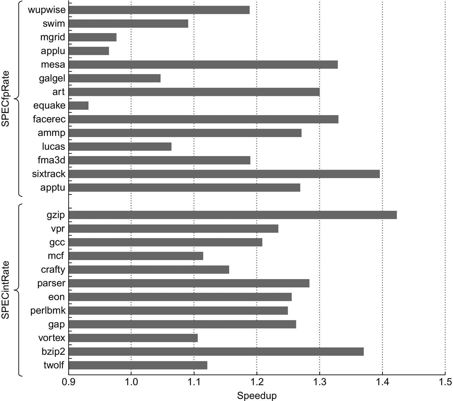
Note that the x-axis starts at a speedup of 0.9, a performance loss. Only one processor in each Power5 core is active, which should slightly improve the results from SMT by decreasing destructive interference in the memory system. The SMT results are obtained by creating 16 user threads, whereas the ST results use only eight threads; with only one thread per processor, the Power5 is switched to single-threaded mode by the OS. These results were collected by John McCalpin at IBM. As we can see from the data, the standard deviation of the results for the SPECfpRate is higher than for SPECintRate (0.13 versus 0.07), indicating that the SMT improvement for FP programs is likely to vary widely.
5.8 Putting It All Together: Multicore Processors and Their Performance
For roughly 10 years, multicore has been the primary focus for scaling performance, although the implementations vary widely, as does their support for larger multichip multiprocessors. In this section, we examine the design of three different multicores, the support they provide for larger multiprocessors, and some performance characteristics, before doing a broader evaluation of small to large multiprocessor Xeon systems, and concluding with a detailed evaluation of the multicore i7 920, a predecessor of the i7 6700.
Performance of Multicore-Based Multiprocessors on a Multiprogrammed Workload
Figure 5.26 shows the key characteristics of three multicore processors designed for server applications and available in 2015 through 2017. The Intel Xeon E7 is based on the same basic design as the i7, but it has more cores, a slightly slower clock rate (power is the limitation), and a larger L3 cache. The Power8 is the newest in the IBM Power series and features more cores and bigger caches. The Fujitsu SPARC64 X + is the newest SPARC server chip; unlike the T-series mentioned in Chapter 3, it uses SMT. Because these processors are configured for multicore and multiprocessor servers, they are available as a family, varying processor count, cache size, and so on, as the figure shows.
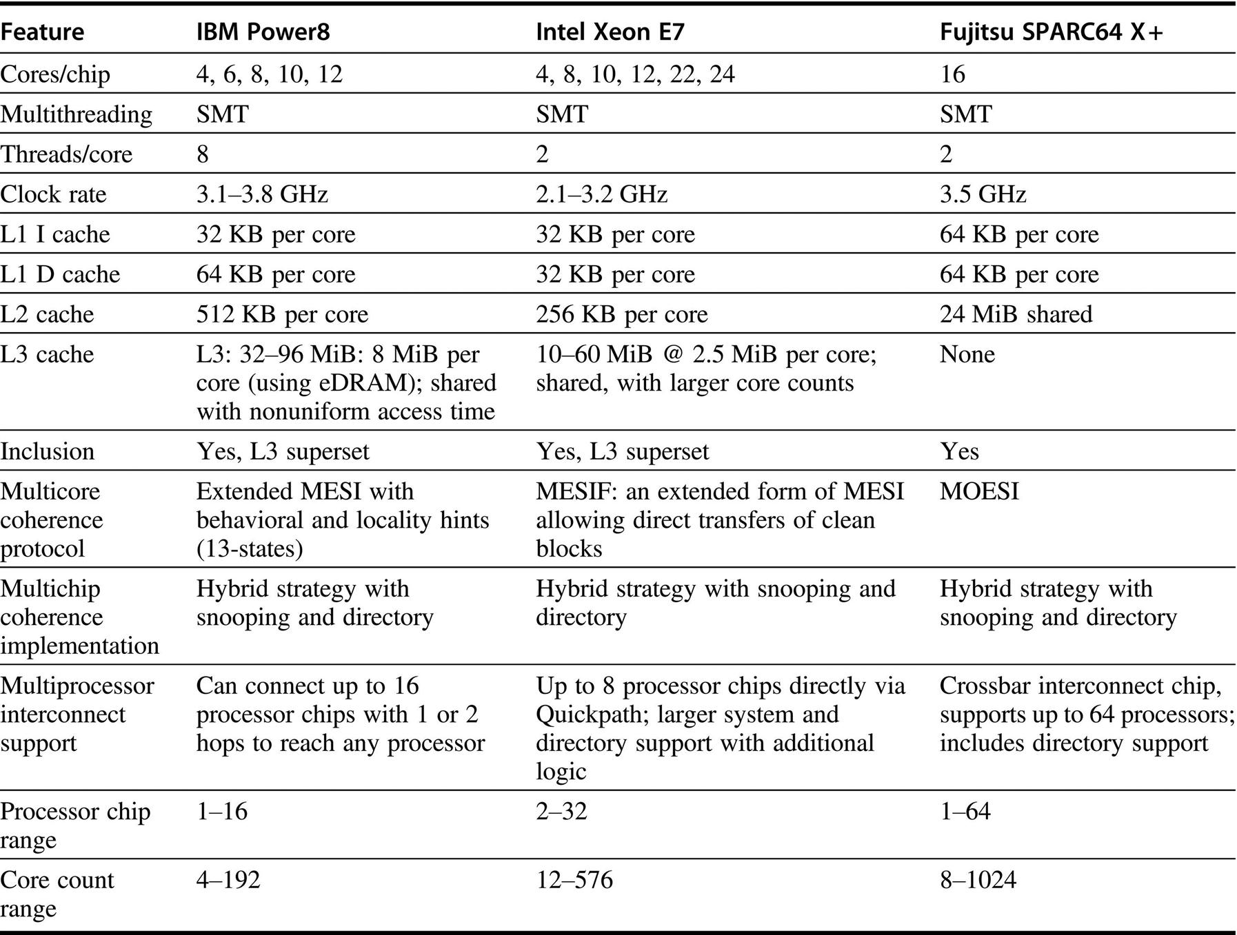
The table shows the range of processor counts, clock rates, and cache sizes within each processor family. The Power8 L3 is a NUCA (Nonuniform Cache Access) design, and it also supports off-chip L4 of up to 128 MiB using EDRAM. A 32-core Xeon has recently been announced, but no system shipments have occurred. The Fujitsu SPARC64 is also available as an 8-core design, which is normally configured as a single processor system. The last row shows the range of configured systems with published performance data (such as SPECintRate) with both processor chip counts and total core counts. The Xeon systems include multiprocessors that extend the basic interconnect with additional logic; for example, using the standard Quickpath interconnect limits the processor count to 8 and the largest system to 8 × 24 = 192 cores, but SGI extends the interconnect (and coherence mechanisms) with extra logic to offer a 32 processor system using 18-core processor chips for a total size of 576 cores. Newer releases of these processors increased clock rates (significantly in the Power8 case, less so in others) and core counts (significantly in the case of Xeon).
These three systems show a range of techniques both for connecting the on-chip cores and for connecting multiple processor chips. First, let's look at how the cores are connected within a chip. The SPARC64 X + is the simplest: it shares a single L2 cache, which is 24-way set associative, among the 16 cores. There are four separate DIMM channels to attach memory accessible with a 16 × 4 switch between the cores and the channels.
Figure 5.27 shows how the Power8 and Xeon E7 chips are organized. Each core in the Power8 has an 8 MiB bank of L3 directly connected; other banks are accessed via the interconnection network, which has 8 separate buses. Thus the Power8 is a true NUCA (Nonuniform Cache Architecture), because the access time to the attached bank of L3 will be much faster than accessing another L3. Each Power8 chip has a set of links that can be used to build a large multiprocessor using an organization we will see shortly. The memory links are connected to a special memory controller that includes an L4 and interfaces directly with DIMMs.
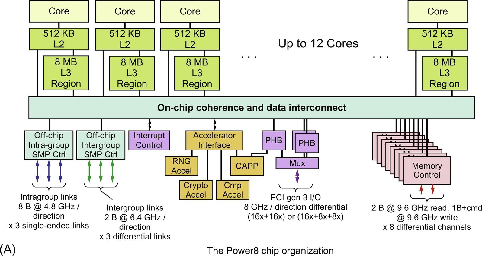
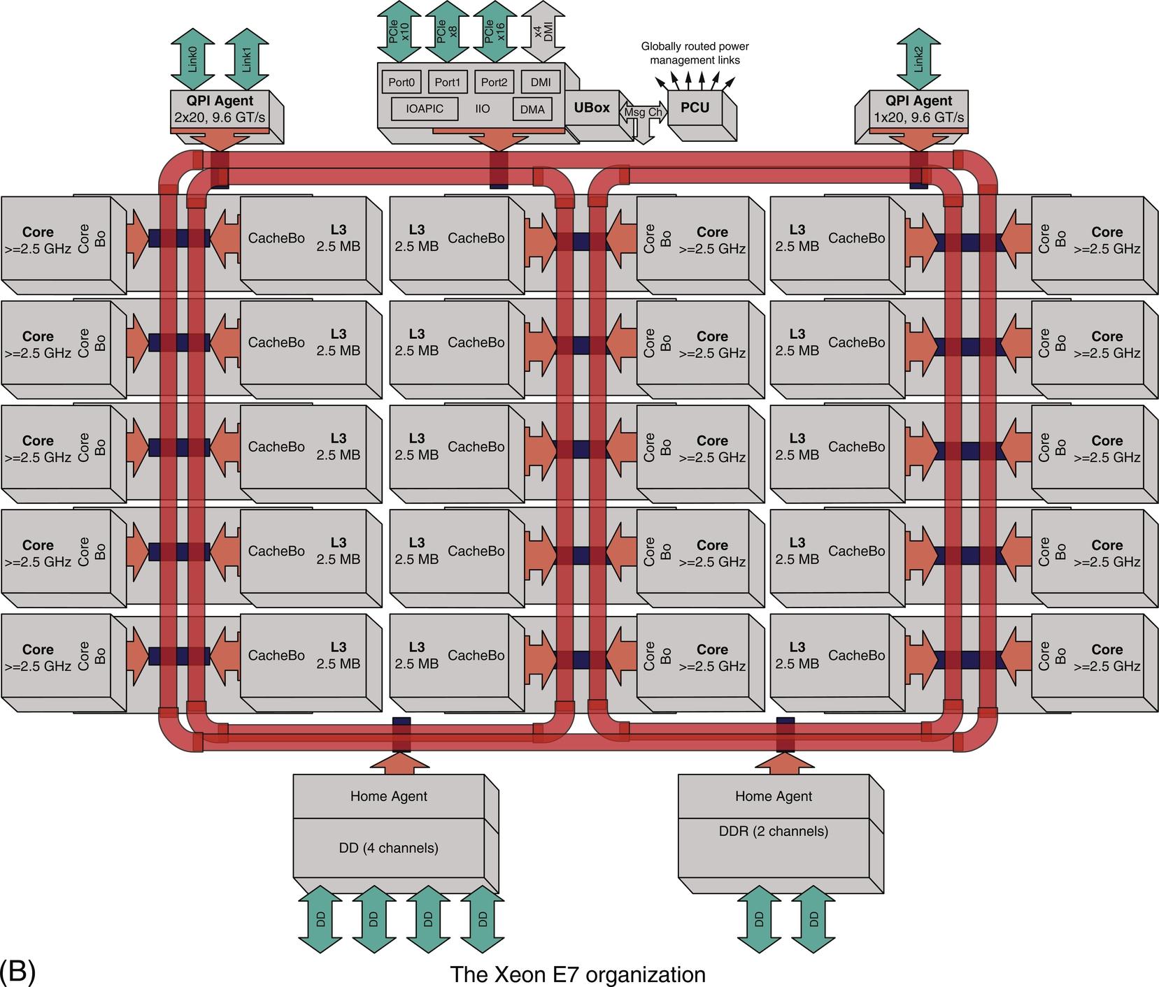
The Power8 uses 8 separate buses between L3 and the CPU cores. Each Power8 also has two sets of links for connecting larger multiprocessors. The Xeon uses three rings to connect processors and L3 cache banks, as well QPI for interchip links. Software is used to logically associate half the cores with each memory channel.
Part B of Figure 5.27, shows how the Xeon E7 processor chip is organized when there are 18 or more cores (20 cores are shown in this figure). Three rings connect the cores and the L3 cache banks, and each core and each bank of L3 is connected to two rings. Thus any cache bank or any core is accessible from any other core by choosing the right ring. Therefore, within the chip, the E7 has uniform access time. In practice, however, the E7 is normally operated as a NUMA architecture by logically associating half the cores with each memory channel; this increases the probability that a desired memory page is open on a given access. The E7 provides 3 QuickPath Interconnect (QPI) links for connecting multiple E7s.
Multiprocessors consisting of these multicores use a variety of different interconnection strategies, as Figure 5.28 shows. The Power8 design provides support for connecting 16 Power8 chips for a total of 192 cores. The intragroup links provide higher bandwidth interconnect among a completely connected module of 4 processor chips. The intergroup links are used to connect each processor chip to the 3 other modules. Thus each processor is two hops from any other, and the memory access time is determined by whether an address resides in local memory, cluster memory, or intercluster memory (actually the latter can have two different values, but the difference is swamped by the intercluster time).
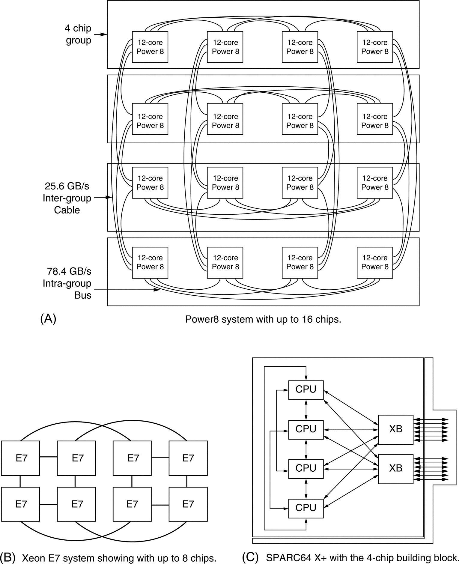
The Xeon E7 uses QPI to interconnect multiple multicore chips. In a 4-chip, multiprocessor, which with the latest announced Xeon could have 128 cores, the three QPI links on each processor are connected to three neighbors, yielding a 4-chip fully connected multiprocessor. Because memory is directly connected to each E7 multicore, even this 4-chip arrangement has nonuniform memory access time (local versus remote). Figure 5.28 shows how 8 E7 processors can be connected; like the Power8, this leads to a situation where every processor is one or two hops from every other processor. There are a number of Xeon-based multiprocessor servers that have more than 8 processor chips. In such designs, the typical organization is to connect 4 processor chips together in a square, as a module, with each processor connecting to two neighbors. The third QPI in each chip is connected to a crossbar switch. Very large systems can be created in this fashion. Memory accesses can then occur at four locations with different timings: local to the processor, an immediate neighbor, the neighbor in the cluster that is two hops away, and through the crossbar. Other organizations are possible and require less than a full crossbar in return for more hops to get to remote memory.
The SPARC64 X + also uses a 4-processor module, but each processor has three connections to its immediate neighbors plus two (or three in the largest configuration) connections to a crossbar. In the largest configuration, 64 processor chips can be connected to two crossbar switches, for a total of 1024 cores. Memory access is NUMA (local, within a module, and through the crossbar), and coherency is directory-based.
Performance of Multicore-Based Multiprocessors on a Multiprogrammed Workload
First, we compare the performance scalability of these three multicore processors using SPECintRate, considering configurations up to 64 cores. Figure 5.29 shows how the performance scales relative to the performance of the smallest configuration, which varies between 4 and 16 cores. In the plot, the smallest configuration is assumed to have perfect speedup (i.e., 8 for 8 cores, 12 for 12 cores, etc.). This figure does not show performance among these different processors. Indeed such performance varies significantly: in the 4-core configuration, the IBM Power8 is 1.5 times as fast as the SPARC64 X + on a per core basis! Instead Figure 5.29 shows how the performance scales for each processor family as additional cores are added.
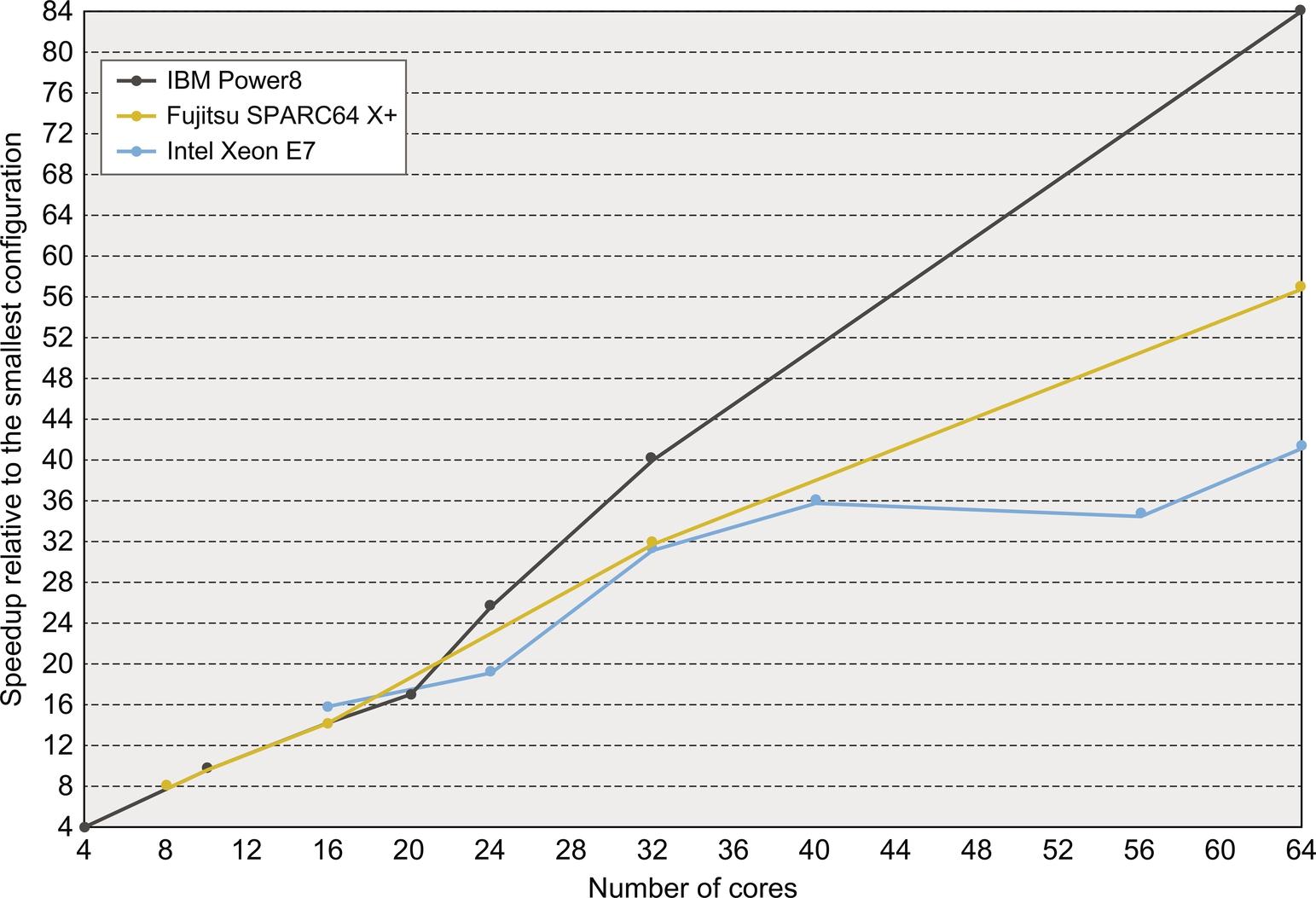
Performance for each processor is plotted relative to the smallest configuration and assuming that configuration had perfect speedup. Although this chart shows how a given multiprocessor scales with additional cores, it does not supply any data about performance among processors. There are differences in the clock rates, even within a given processor family. These are generally swamped by the core scaling effects, except for the Power8 that shows a clock range spread of 1.5 × from the smallest configuration to the 64 core configuration.
Two of the three processors show diminishing returns as they scale to 64 cores. The Xeon systems appear to show the most degradation at 56 and 64 cores. This may be largely due to having more cores share a smaller L3. For example, the 40-core system uses 4 chips, each with 60 MiB of L3, yielding 6 MiB of L3 per core. The 56-core and 64-core systems also use 4 chips but have 35 or 45 MiB of L3 per chip, or 2.5–2.8 MiB per core. It is likely that the resulting larger L3 miss rates lead to the reduction in speedup for the 56-core and 64-core systems.
The IBM Power8 results are also unusual, appearing to show significant superlinear speedup. This effect, however, is due largely to differences in the clock rates, which are much larger across the Power8 processors than for the other processors in this figure. In particular, the 64-core configuration has the highest clock rate (4.4 GHz), whereas the 4-core configuration has a 3.0 GHz clock. If we normalize the relative speedup for the 64-core system based on the clock rate differential with the 4-core system, the effective speedup is 57 rather than 84. Therefore, while the Power8 system scales well, and perhaps the best among these processors, it is not miraculous.
Figure 5.30 shows scaling for these three systems at configurations above 64 processors. Once again, the clock rate differential explains the Power8 results; the clock-rate equivalent scaled speedup with 192 processors is 167, versus 223, when not accounting for clock rate differences. Even at 167, the Power8 scaling is somewhat better than that on the SPARC64 X + or Xeon systems. Surprisingly, although there are some effects on speedup in going from the smallest system to 64 cores, they do not seem to get dramatically worse at these larger configurations. The nature of the workload, which is highly parallel and user-CPU-intensive, and the overheads paid in going to 64 cores probably lead to this result.
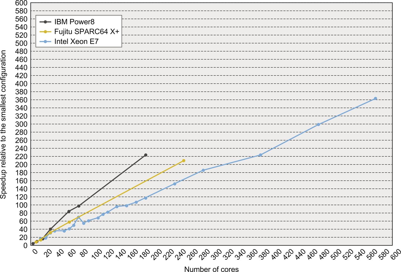
As before, performance is shown relative to the smallest available system. The Xeon result at 80 cores is the same L3 effect that showed up for smaller configurations. All systems larger than 80 cores have between 2.5 and 3.8 MiB of L3 per core, and the 80-core, or smaller, systems have 6 MiB per core.
Scalability in an Xeon MP With Different Workloads
In this section, we focus on the scalability of the Xeon E7 multiprocessors on three different workloads: a Java-based commercially oriented workload, a virtual machine workload, and a scientific parallel processing workload, all from the SPEC benchmarking organization, as described next.
- SPECjbb2015: Models a supermarket IT system that handles a mix of point-of-sale requests, online purchases, and data-mining operations. The performance metric is throughput-oriented, and we use the maximum performance measurement on the server side running multiple Java virtual machines.
- SPECVirt2013: Models a collection of virtual machines running independent mixes of other SPEC benchmarks, including CPU benchmarks, web servers, and mail servers. The system must meet a quality of service guarantee for each virtual machine.
- SPECOMP2012: A collection of 14 scientific and engineering programs written with the OpenMP standard for shared-memory parallel processing. The codes are written in Fortran, C, and C++ and range from fluid dynamics to molecular modeling to image manipulation.
As with the previous results, Figure 5.31 shows performance assuming linear speedup on the smallest configuration, which for these benchmarks varies from 48 cores to 72 cores, and plotting performance relative to the that smallest configuration. The SPECjbb2015 and SPECVirt2013 include significant systems software, including the Java VM software and the VM hypervisor. Other than the system software, the interaction among the processes is very small. In contrast, SPECOMP2012 is a true parallel code with multiple user processes sharing data and collaborating in the computation.
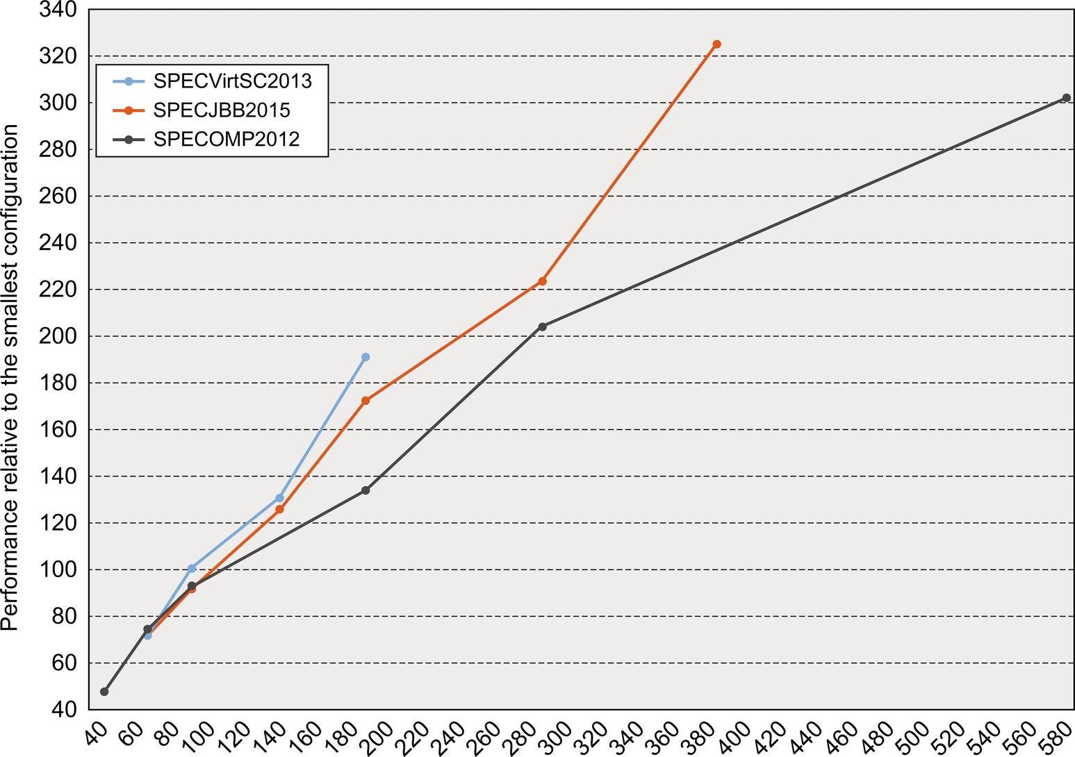
Only relative performance can be assessed from this data, and comparisons across the benchmarks have no relevance. Note the difference in the scale of the vertical and horizontal axes.
Let's begin by examining SPECjbb2015. It obtains speedup efficiency (speedup/processor ratio) of between 78% and 95%, showing good speedup, even in the largest configuration. SPECVirt2013 does even better (for the range of system measured), obtaining almost linear speedup at 192 cores. Both SPECjbb2015 and SPECVirt2013 are benchmarks that scale up the application size (as in the TPC benchmarks discussed in Chapter 1) with larger systems so that the effects of Amdahl's Law and interprocess communication are minor.
Finally, let's turn to SPECOMP2012, the most compute-intensive of these benchmarks and the one that truly involves parallel processing. The major trend visible here is a steady loss of efficiency as we scale from 30 to 576 cores so that by 576 cores, the system exhibits only half the efficiency it showed at 30 cores. This reduction leads to a relative speedup of 284, assuming that the 30-core speedup is 30. These are probably Amdahl's Law effects resulting from limited parallelism as well as synchronization and communication overheads. Unlike the SPECjbb2015 and SPECVirt2013, these benchmarks are not scaled for larger systems.
Performance and Energy Efficiency of the Intel i7 920 Multicore
In this section, we closely examine the performance of the i7 920, a predecessor of the 6700, on the same two groups of benchmarks we considered in Chapter 3: the parallel Java benchmarks and the parallel PARSEC benchmarks (described in detail in Figure 3.32 on page 247). Although this study uses the older i7 920, it remains, by far, the most comprehensive study of energy efficiency in multicore processors and the effects of multicore combined with SMT. The fact that the i7 920 and 6700 are similar indicates that the basic insights should also apply to the 6700.
First, we look at the multicore performance and scaling versus a single-core without the use of SMT. Then we combine both the multicore and SMT capability. All the data in this section, like that in the earlier i7 SMT evaluation (Chapter 3) come from Esmaeilzadeh et al. (2011). The dataset is the same as that used earlier (see Figure 3.32 on page 247), except that the Java benchmarks tradebeans and pjbb2005 are removed (leaving only the five scalable Java benchmarks); tradebeans and pjbb2005 never achieve speedup above 1.55 even with four cores and a total of eight threads, and thus are not appropriate for evaluating more cores.
Figure 5.32 plots both the speedup and energy efficiency of the Java and PARSEC benchmarks without the use of SMT. Energy efficiency is computed by the ratio: energy consumed by the single-core run divided by the energy consumed by the two- or four-core run (i.e., efficiency is the inverse of energy consumed). Higher energy efficiency means that the processor consumes less energy for the same computation, with a value of 1.0 being the break-even point. The unused cores in all cases were in deep sleep mode, which minimized their power consumption by essentially turning them off. In comparing the data for the single-core and multicore benchmarks, it is important to remember that the full energy cost of the L3 cache and memory interface is paid in the single-core (as well as the multicore) case. This fact increases the likelihood that energy consumption will improve for applications that scale reasonably well. Harmonic mean is used to summarize results with the implication described in the caption.
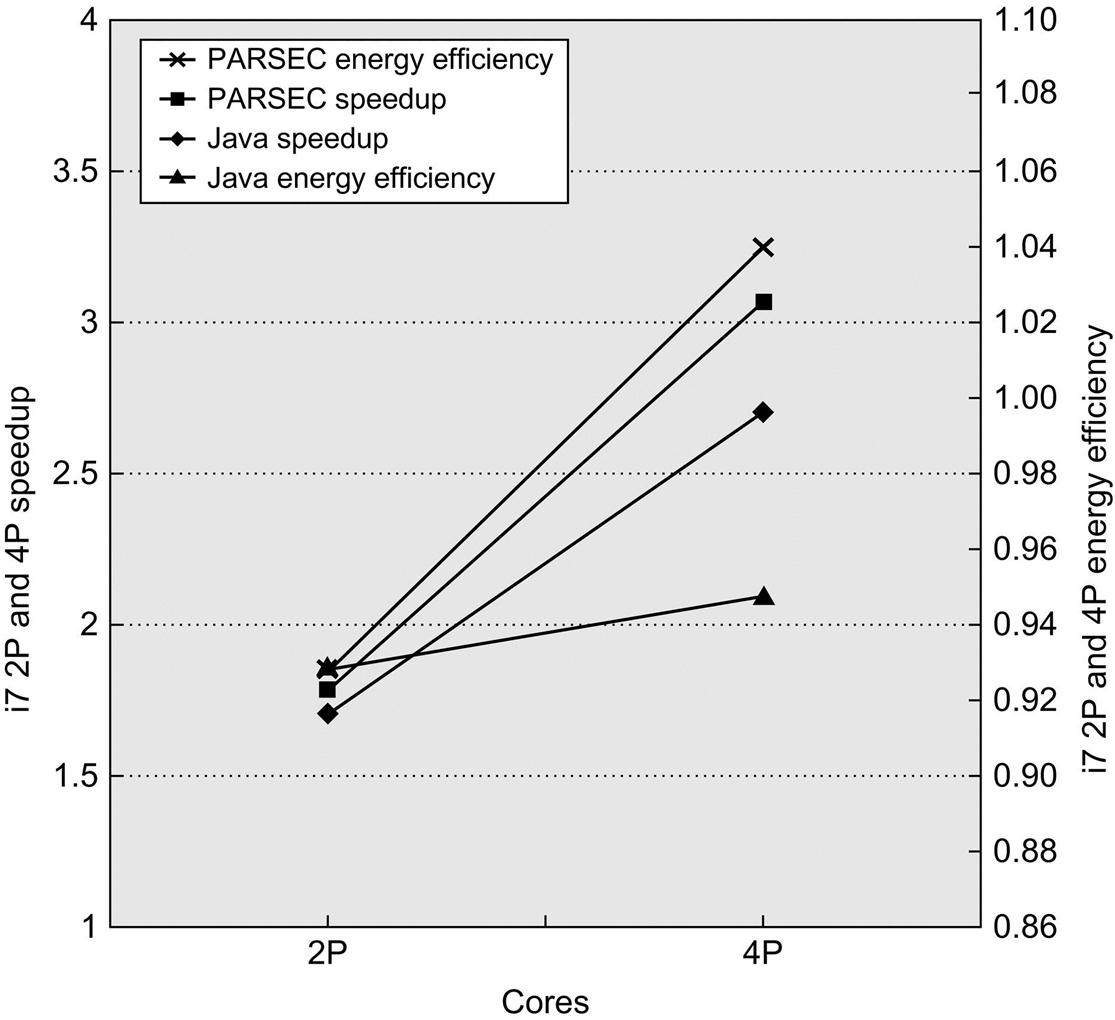
These data were collected by Esmaeilzadeh et al. (2011) using the same setup as described in Chapter 3. Turbo Boost is turned off. The speedup and energy efficiency are summarized using harmonic mean, implying a workload where the total time spent running each benchmark on 2 cores is equivalent.
As the figure shows, the PARSEC benchmarks get better speedup than the Java benchmarks, achieving 76% speedup efficiency (i.e., actual speedup divided by processor count) on four cores, whereas the Java benchmarks achieve 67% speedup efficiency on four cores. Although this observation is clear from the data, analyzing why this difference exists is difficult. It is quite possible that Amdahl's Law effects have reduced the speedup for the Java workload, which includes some typically serial parts, such as the garbage collector. In addition, interaction between the processor architecture and the application, which affects issues such as the cost of synchronization or communication, may also play a role. In particular, well-parallelized applications, such as those in PARSEC, sometimes benefit from an advantageous ratio between computation and communication, which reduces the dependence on communications costs (see Appendix I).
These differences in speedup translate to differences in energy efficiency. For example, the PARSEC benchmarks actually slightly improve energy efficiency over the single-core version; this result may be significantly affected by the fact that the L3 cache is more effectively used in the multicore runs than in the single-core case and the energy cost is identical in both cases. Thus, for the PARSEC benchmarks, the multicore approach achieves what designers hoped for when they switched from an ILP-focused design to a multicore design; namely, it scales performance as fast or faster than scaling power, resulting in constant or even improved energy efficiency. In the Java case, we see that neither the two- nor four-core runs break even in energy efficiency because of the lower speedup levels of the Java workload (although Java energy efficiency for the 2p run is the same as for PARSEC). The energy efficiency in the four-core Java case is reasonably high (0.94). It is likely that an ILP-centric processor would need even more power to achieve a comparable speedup on either the PARSEC or Java workload. Thus the TLP-centric approach is also certainly better than the ILP-centric approach for improving performance for these applications. As we will see in Section 5.10, there are reasons to be pessimistic about simple, efficient, long-term scaling of multicore.
Putting Multicore and SMT Together
Finally, we consider the combination of multicore and multithreading by measuring the two benchmark sets for two to four processors and one to two threads (a total of four data points and up to eight threads). Figure 5.33 shows the speedup and energy efficiency obtained on the Intel i7 when the processor count is two or four and SMT is or is not employed, using harmonic mean to summarize the two benchmarks sets. Clearly, SMT can add to performance when there is sufficient thread-level parallelism available even in the multicore situation. For example, in the four-core, no-SMT case, the speedup efficiencies were 67% and 76% for Java and PARSEC, respectively. With SMT on four cores, those ratios are an astonishing 83% and 97%.
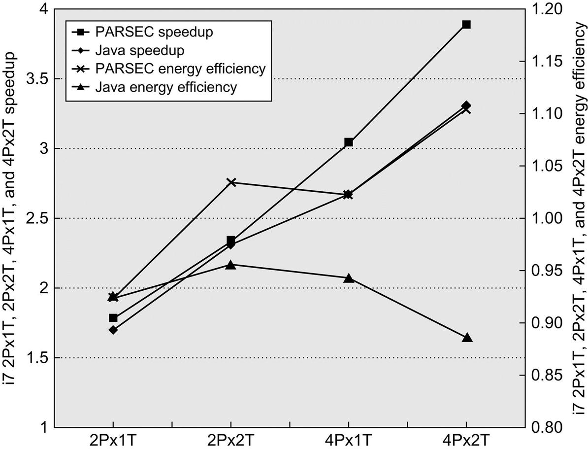
Remember that the preceding results vary in the number of threads from two to eight and reflect both architectural effects and application characteristics. Harmonic mean is used to summarize results, as discussed in the Figure 5.32 caption.
Energy efficiency presents a slightly different picture. In the case of PARSEC, speedup is essentially linear for the four-core SMT case (eight threads), and power scales more slowly, resulting in an energy efficiency of 1.1 for that case. The Java situation is more complex; energy efficiency peaks for the two-core SMT (four-thread) run at 0.97 and drops to 0.89 in the four-core SMT (eight-thread) run. It seems highly likely that the Java benchmarks are encountering Amdahl's Law effects when more than four threads are deployed. As some architects have observed, multicore does shift more responsibility for performance (and thus energy efficiency) to the programmer, and the results for the Java workload certainly bear this out.
5.9 Fallacies and Pitfalls
Given the lack of maturity in our understanding of parallel computing, there are many hidden pitfalls that will be uncovered either by careful designers or by unfortunate ones. Given the large amount of hype that has surrounded multiprocessors over the years, common fallacies abound. We have included a selection of them.
- Pitfall Measuring performance of multiprocessors by linear speedup versus execution time.
Graphs like those in Figures 5.32 and 5.33, which plot performance versus number of processors, showing linear speedup, a plateau, and then a falling off, have long been used to judge the success of parallel processors. Although speedup is one facet of a parallel program, it is not a direct measure of performance. The first issue is the power of the processors being scaled: a program that linearly improves performance to equal 100 Intel Atom processors (the low-end processor used for netbooks) may be slower than the version run on an 8-core Xeon. Be especially careful of floating-point-intensive programs; processing elements without hardware assist may scale wonderfully but have poor collective performance.
Comparing execution times is fair only if you are comparing the best algorithms on each computer. Comparing the identical code on two computers may seem fair, but it is not; the parallel program may be slower on a uniprocessor than on a sequential version. Developing a parallel program will sometimes lead to algorithmic improvements, so comparing the previously best-known sequential program with the parallel code—which seems fair—will not compare equivalent algorithms. To reflect this issue, the terms relative speedup (same program) and true speedup (best program) are sometimes used.
Results that suggest superlinear performance, when a program on n processors is more than n times faster than the equivalent uniprocessor, may indicate that the comparison is unfair, although there are instances where “real” superlinear speedups have been encountered. For example, some scientific applications regularly achieve superlinear speedup for small increases in processor count (2 or 4 to 8 or 16). These results usually arise because critical data structures that do not fit into the aggregate caches of a multiprocessor with 2 or 4 processors fit into the aggregate cache of a multiprocessor with 8 or 16 processors. As we saw in the previous section, other differences (such as high clock rate) may appear to yield superlinear speedups when comparing slightly different systems.
In summary, comparing performance by comparing speedups is at best tricky and at worst misleading. Comparing the speedups for two different multiprocessors does not necessarily tell us anything about the relative performance of the multiprocessors, as we also saw in the previous section. Even comparing two different algorithms on the same multiprocessor is tricky because we must use true speedup, rather than relative speedup, to obtain a valid comparison.
- Fallacy Amdahl's Law doesn't apply to parallel computers.
In 1987 the head of a research organization claimed that Amdahl's Law (see Section 1.9) had been broken by an MIMD multiprocessor. This statement hardly meant, however, that the law has been overturned for parallel computers; the neglected portion of the program will still limit performance. To understand the basis of the media reports, let's see what Amdahl (1967) originally said:A fairly obvious conclusion which can be drawn at this point is that the effort expended on achieving high parallel processing rates is wasted unless it is accompanied by achievements in sequential processing rates of very nearly the same magnitude. [p. 483]
One interpretation of the law was that, because portions of every program must be sequential, there is a limit to the useful economic number of processors—say, 100. By showing linear speedup with 1000 processors, this interpretation of Amdahl's Law was disproved.
The basis for the statement that Amdahl's Law had been “overcome” was the use of scaled speedup, also called weak scaling. The researchers scaled the benchmark to have a dataset size that was 1000 times larger and compared the uniprocessor and parallel execution times of the scaled benchmark. For this particular algorithm, the sequential portion of the program was constant independent of the size of the input, and the rest was fully parallel—thus, linear speedup with 1000 processors. Because the running time grew faster than linear, the program actually ran longer after scaling, even with 1000 processors.
Speedup that assumes scaling of the input is not the same as true speedup, and reporting it as if it were is misleading. Because parallel benchmarks are often run on different-sized multiprocessors, it is important to specify what type of application scaling is permissible and how that scaling should be done. Although simply scaling the data size with processor count is rarely appropriate, assuming a fixed problem size for a much larger processor count (called strong scaling) is often inappropriate, as well, because it is likely that users given a much larger multiprocessor would opt to run a larger or more detailed version of an application. See Appendix I for more discussion on this important topic.
- Fallacy Linear speedups are needed to make multiprocessors cost-effective.
It is widely recognized that one of the major benefits of parallel computing is to offer a “shorter time to solution” than the fastest uniprocessor. Many people, however, also hold the view that parallel processors cannot be as cost-effective as uniprocessors unless they can achieve perfect linear speedup. This argument says that, because the cost of the multiprocessor is a linear function of the number of processors, anything less than linear speedup means that the performance/cost ratio decreases, making a parallel processor less cost-effective than using a uniprocessor.
The problem with this argument is that cost is not only a function of processor count but also depends on memory, I/O, and the overhead of the system (box, power supply, interconnect, etc.). It also makes less sense in the multicore era, when there are multiple processors per chip.
The effect of including memory in the system cost was pointed out by Wood and Hill (1995). We use an example based on more recent data using TPC-C and SPECRate benchmarks, but the argument could also be made with a parallel scientific application workload, which would likely make the case even stronger.
Figure 5.34 shows the speedup for TPC-C, SPECintRate, and SPECfpRate on an IBM eServer p5 multiprocessor configured with 4–64 processors. The figure shows that only TPC-C achieves better than linear speedup. For SPECintRate and SPECfpRate, speedup is less than linear, but so is the cost, because unlike TPC-C, the amount of main memory and disk required both scale less than linearly.
As Figure 5.35 shows, larger processor counts can actually be more cost-effective than the 4-processor configuration. In comparing the cost-performance of two computers, we must be sure to include accurate assessments of both total system cost and what performance is achievable. For many applications with larger memory demands, such a comparison can dramatically increase the attractiveness of using a multiprocessor.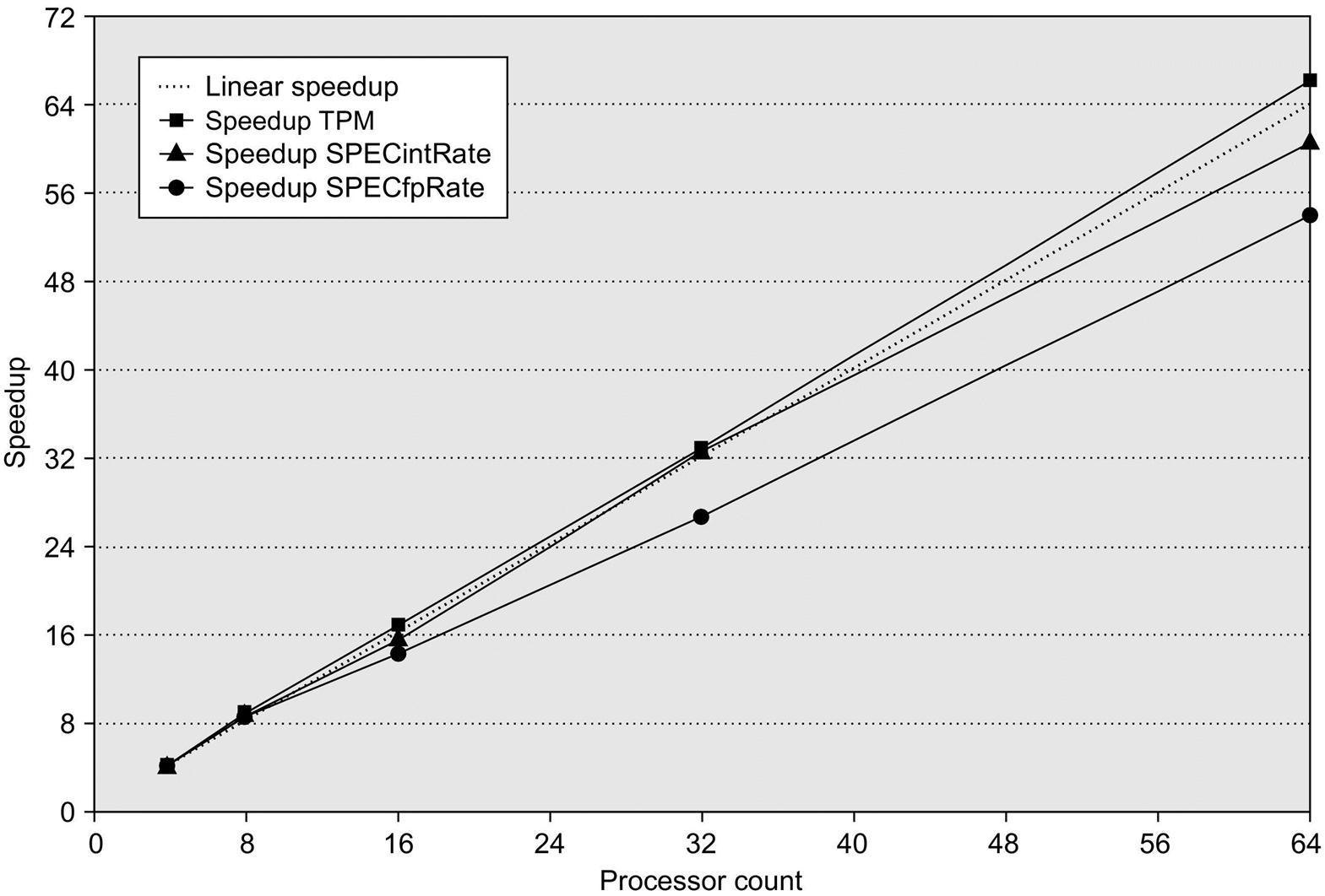
Figure 5.34 Speedup for three benchmarks on an IBM eServer p5 multiprocessor when configured with 4, 8, 16, 32, and 64 processors.
The dashed line shows linear speedup.
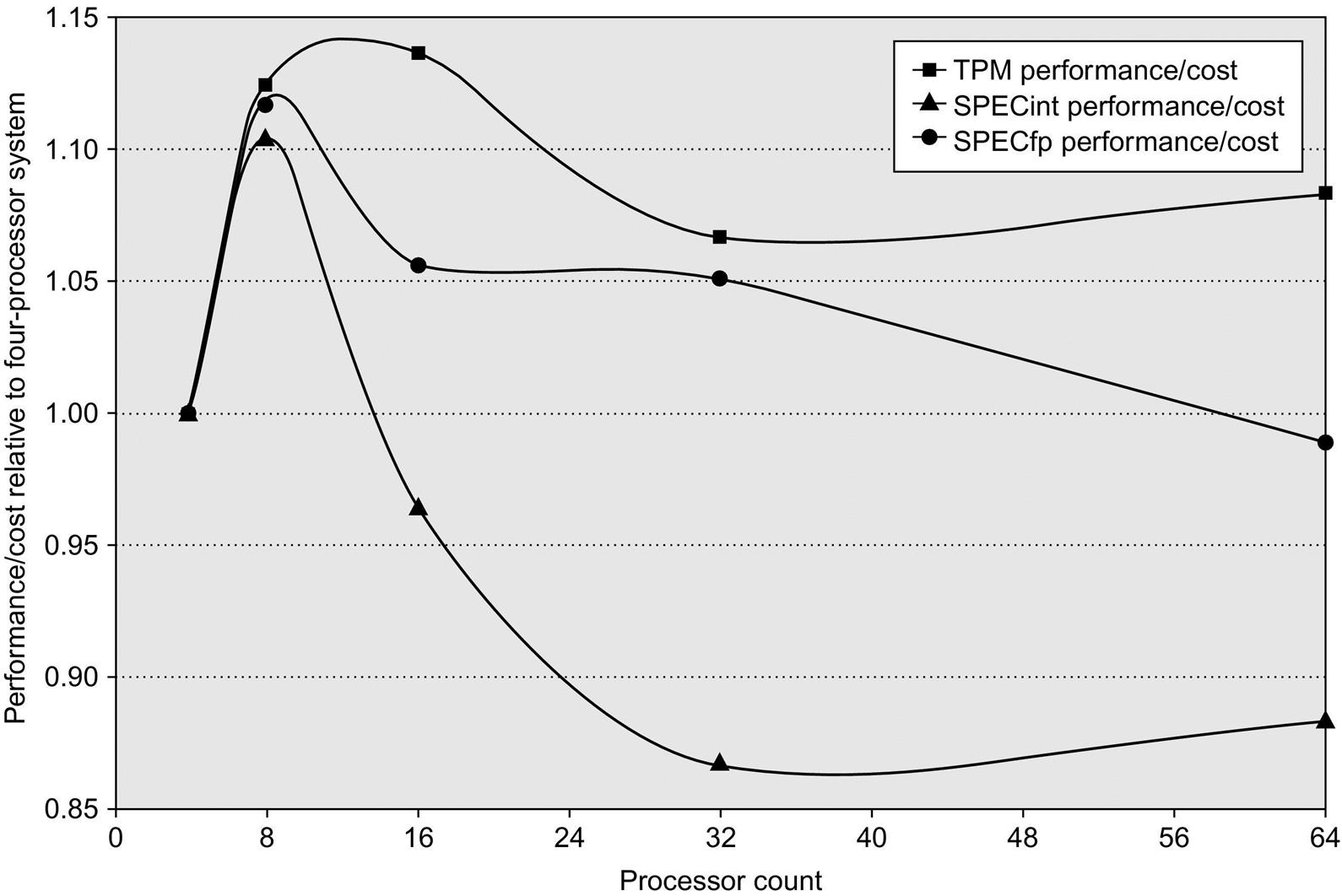
Any measurement above 1.0 indicates that the configuration is more cost-effective than the 4-processor system. The 8-processor configurations show an advantage for all three benchmarks, whereas two of the three benchmarks show a cost-performance advantage in the 16- and 32-processor configurations. For TPC-C, the configurations are those used in the official runs, which means that disk and memory scale nearly linearly with processor count, and a 64-processor machine is approximately twice as expensive as a 32-processor version. In contrast, the disk and memory are scaled more slowly (although still faster than necessary to achieve the best SPECRate at 64 processors). In particular, the disk configurations go from one drive for the 4-processor version to four drives (140 GB) for the 64-processor version. Memory is scaled from 8 GiB for the 4-processor system to 20 GiB for the 64-processor system.
- Pitfall Not developing the software to take advantage of, or optimize for, a multiprocessor architecture.
There is a long history of software lagging behind on multiprocessors, probably because the software problems are much harder. We give one example to show the subtlety of the issues, but there are many examples we could choose from.
One frequently encountered problem occurs when software designed for a uniprocessor is adapted to a multiprocessor environment. For example, the SGI operating system in 2000 originally protected the page table data structure with a single lock, assuming that page allocation was infrequent. In a uniprocessor, this does not represent a performance problem. In a multiprocessor, it can become a major performance bottleneck for some programs.
Consider a program that uses a large number of pages that are initialized at startup, which UNIX does for statically allocated pages. Suppose the program is parallelized so that multiple processes allocate the pages. Because page allocation requires the use of the page table data structure, which is locked whenever it is in use, even an OS kernel that allows multiple threads in the OS will be serialized if the processes all try to allocate their pages at once (which is exactly what we might expect at initialization time).
This page table serialization eliminates parallelism in initialization and has significant impact on overall parallel performance. This performance bottleneck persists even under multiprogramming. For example, suppose we split the parallel program apart into separate processes and run them, one process per processor, so that there is no sharing between the processes. (This is exactly what one user did, because he reasonably believed that the performance problem was due to unintended sharing or interference in his application.) Unfortunately, the lock still serializes all the processes, so even the multiprogramming performance is poor. This pitfall indicates the kind of subtle but significant performance bugs that can arise when software runs on multiprocessors. Like many other key software components, the OS algorithms and data structures must be rethought in a multiprocessor context. Placing locks on smaller portions of the page table effectively eliminates the problem. Similar problems exist in memory structures, which increases the coherence traffic in cases where no sharing is actually occurring.
As multicore became the dominant theme in everything from desktops to servers, the lack of an adequate investment in parallel software became apparent. Given the lack of focus, it will likely be many years before the software systems we use adequately exploit the growing numbers of cores.
5.10 The Future of Multicore Scaling
For more than 30 years, researchers and designers have predicted the end of uniprocessors and their dominance by multiprocessors. Until the early years of this century, this prediction was constantly proven wrong. As we saw in Chapter 3, the costs of trying to find and exploit more ILP became prohibitive in efficiency (both in silicon area and in power). Of course, multicore does not magically solve the power problem because it clearly increases both the transistor count and the active number of transistors switching, which are the two dominant contributions to power. As we will see in this section, energy issues are likely to limit multicore scaling more severely than previously thought.
ILP scaling failed because of both limitations in the ILP available and the efficiency of exploiting that ILP. Similarly, a combination of two factors means that simply scaling performance by adding cores is unlikely to be broadly successful. This combination arises from the challenges posed by Amdahl's Law, which assesses the efficiency of exploiting parallelism, and the end of Dennard's Scaling, which dictates the energy required for a multicore processor.
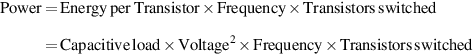
To understand these factors, we take a simple model of both technology scaling (based on an extensive and highly detailed analysis in Esmaeilzadeh et al. (2012)). Let's start by reviewing energy consumption and power in CMOS. Recall from Chapter 1 that the energy to switch a transistor is given as

CMOS scaling is limited primarily by thermal power, which is a combination of static leakage power and dynamic power, which tends to dominate. Power is given by
To understand the implications of how energy and power scale, let's compare today's 22 nm technology with a technology projected to be available in 2021–24 (depending on the rate at which Moore's Law continues to slow down). Figure 5.36 shows this comparison based on technology projections and resulting effects on energy and power scaling. Notice that power scaling > 1.0 means that the future device consumes more power; in this case, 1.79 × as much.
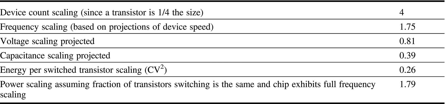
The characteristics of the 11 nm technology are based on the International Technology Roadmap for Semiconductors, which has been recently discontinued because of uncertainty about the continuation of Moore's Law and what scaling characteristics will be seen.
Consider the implications of this for one of the latest Intel Xeon processors, the E7-8890, which has 24 cores, 7.2 billion transistors (including almost 70 MiB of cache), operates at 2.2 GHz, has a thermal power rating of 165 watts, and a die size of 456 mm2. The clock frequency is already limited by power dissipation: a 4-core version has a clock of 3.2 GHz, and a 10-core version has a 2.8 GHz clock. With the 11 nm technology, the same size die would accommodate 96 cores with almost 280 MiB of cache and operate at a clock rate (assuming perfect frequency scaling) of 4.9 GHz. Unfortunately, with all cores operating and no efficiency improvements, it would consume 165 × 1.79 = 295 watts. If we assume the 165-W heat dissipation limit remains, then only 54 cores can be active. This limit yields a maximum performance speedup of 54/24 = 2.25 over a 5–6 year period, less than one-half the performance scaling seen in the late 1990s. Furthermore, we may have Amdahl's Law effects, as the next example shows.
Example
Suppose we have a 96-core future generation processor, but on average only 54 cores can be busy. Suppose that 90% of the time, we can use all available cores; 9% of the time, we can use 50 cores; and 1% of the time is strictly serial. How much speedup might we expect? Assume that cores can be turned off when not in use and draw no power and assume that the use of a different number of cores is distributed so that we need to worry only about average power consumption. How would the multicore speedup compare to the 24-processor count version that can use all its processor 99% of the time?
Answer
We can find how many cores can be used for the 90% of the time when more than 54 are usable, as follows:
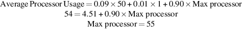
Now, we can find the speedup:
Now compute the speedup on 24 processors:
When considering both power constraints and Amdahl's Law effects, the 96-processor version achieves less than a factor of 2 speedup over the 24-processor version. In fact, the speedup from clock rate increase nearly matches the speedup from the 4 × processor count increase. We comment on these issues further in the concluding remarks.
5.11 Concluding Remarks
As we saw in the previous section, multicore does not magically solve the power problem because it clearly increases both the transistor count and the active number of transistors switching, which are the two dominant contributions to power. The failure of Dennard scaling merely makes it more extreme.
But multicore does alter the game. By allowing idle cores to be placed in power-saving mode, some improvement in power efficiency can be achieved, as the results in this chapter have shown. For example, shutting down cores in the Intel i7 allows other cores to operate in Turbo mode. This capability allows a trade-off between higher clock rates with fewer processors and more processors with lower clock rates.
More importantly, multicore shifts the burden for keeping the processor busy by relying more on TLP, which the application and programmer are responsible for identifying, rather than on ILP, for which the hardware is responsible. Multiprogrammed and highly parallel workloads that avoid Amdahl's Law effects will benefit more easily.
Although multicore provides some help with the energy efficiency challenge and shifts much of the burden to the software system, there remain difficult challenges and unresolved questions. For example, attempts to exploit thread-level versions of aggressive speculation have so far met the same fate as their ILP counterparts. That is, the performance gains have been modest and are likely less than the increase in energy consumption, so ideas such as speculative threads or hardware run-ahead have not been successfully incorporated in processors. As in speculation for ILP, unless the speculation is almost always right, the costs exceed the benefits.
Thus, at the present, it seems unlikely that some form of simple multicore scaling will provide a cost-effective path to growing performance. A fundamental problem must be overcome: finding and exploiting significant amounts of parallelism in an energy- and silicon-efficient manner. In the previous chapter, we examined the exploitation of data parallelism via a SIMD approach. In many applications, data parallelism occurs in large amounts, and SIMD is a more energy-efficient method for exploiting data parallelism. In the next chapter, we explore large-scale cloud computing. In such environments, massive amounts of parallelism are available from millions of independent tasks generated by individual users. Amdahl's Law plays little role in limiting the scale of such systems because the tasks (e.g., millions of Google search requests) are independent. Finally, in Chapter 7, we explore the rise of domain-specific architectures (DSAs). Most domain-specific architectures exploit the parallelism of the targeted domain, which is often data parallelism, and as with GPUs, DSAs can achieve much higher efficiency as measured by energy consumption or silicon utilization.
In the last edition, published in 2012, we raised the question of whether it would be worthwhile to consider heterogeneous processors. At that time, no such multicore was delivered or announced, and heterogeneous multiprocessors had seen only limited success in special-purpose computers or embedded systems. While the programming models and software systems remain challenging, it appears inevitable that multiprocessors with heterogeneous processors will play an important role. Combining domain-specific processors, like those discussed in Chapters 4 and 7, with general-purpose processors is perhaps the best road forward to achieve increased performance and energy efficiency while maintaining some of the flexibility that general-purpose processors offer.
5.12 Historical Perspectives and References
Section M.7 (available online) looks at the history of multiprocessors and parallel processing. Divided by both time period and architecture, the section features discussions on early experimental multiprocessors and some of the great debates in parallel processing. Recent advances are also covered. References for further reading are included.
Case Studies and Exercises by Amr Zaky and David A. Wood
Case Study 1: Single Chip Multicore Multiprocessor
Concepts illustrated by this case study
A multicore SMT multiprocessor is illustrated in Figure 5.37. Only the cache contents are shown. Each core has a single, private cache with coherence maintained using the snooping coherence protocol of Figure 5.7. Each cache is direct-mapped, with four lines, each holding 2 bytes (to simplify diagram). For further simplification, the whole line addresses in memory are shown in the address fields in the caches, where the tag would normally exist. The coherence states are denoted M, S, and I for Modified, Shared, and Invalid.
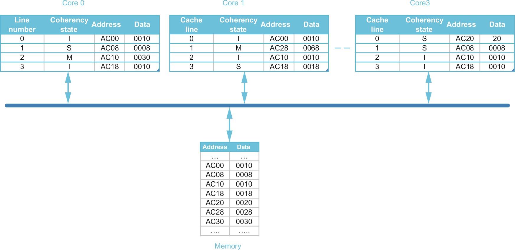
- 5.1. [10/10/10/10/10/10/10] <5.2> For each part of this exercise, the initial cache and memory state are assumed to initially have the contents shown in Figure 5.37. Each part of this exercise specifies a sequence of one or more CPU operations of the form
Ccore#: R, < address > for reads
and
Ccore#: W, < address > <-- < value written > for writes.
For example,
C3: R, AC10 & C0: W, AC18 <-- 0018
Read and write operations are for 1 byte at a time. Show the resulting state (i.e., coherence state, tags, and data) of the caches and memory after the actions given below. Show only the cache lines that experience some state change; for example:
C0.L0: (I, AC20, 0001) indicates that line 0 in core 0 assumes an “invalid” coherence state (I), stores AC20 from the memory, and has data contents 0001. Furthermore, represent any changes to the memory state as M: < address > <-- value.
Different parts (a) through (g) do not depend on one another: assume the actions in all parts are applied to the initial cache and memory states. - 5.2. [20/20/20/20] <5.3> The performance of a snooping cache-coherent multiprocessor depends on many detailed implementation issues that determine how quickly a cache responds with data in an exclusive or M state block. In some implementations, a processor read miss to a cache block that is exclusive in another processor's cache is faster than a miss to a block in memory. This is because caches are smaller, and thus faster, than main memory. Conversely, in some implementations, misses satisfied by memory are faster than those satisfied by caches. This is because caches are generally optimized for “front side” or CPU references, rather than “back side” or snooping accesses. For the multiprocessor illustrated in Figure 5.37, consider the execution of a sequence of operations on a single processor core where
- read and write hits generate no stall cycles;
- read and write misses generate Nmemory and Ncache stall cycles if satisfied by memory and cache, respectively;
- write hits that generate an invalidate incur Ninvalidate stall cycles; and
- a write-back of a block, either due to a conflict or another processor's request to an exclusive block, incurs an additional Nwriteback stall cycles.
Consider two implementations with different performance characteristics summarized in Figure 5.38.
To observe how these cycle values are used, we illustrate how the following sequence of operations, assuming the initial caches' states in Figure 5.37, behave under implementation 1.
C1: R, AC10
C3: R, AC10
For simplicity, assume that the second operation begins after the first completes, even though they are on different processor cores.
For Implementation 1,- the first read generates 50 stall cycles because the read is satisfied by C0's cache: C1 stalls for 40 cycles while it waits for the block, and C0 stalls for 10 cycles while it writes the block back to memory in response to C1's request; and
- the second read by C3 generates 100 stall cycles because its miss is satisfied by memory.
Therefore this sequence generates a total of 150 stall cycles.
For the following sequences of operations, how many stall cycles are generated by each implementation? - 5.3. [20] <5.2> Some applications read a large dataset first and then modify most or all of it. The base MSI coherence protocol will first fetch all of the cache blocks in the Shared state and then be forced to perform an invalidate operation to upgrade them to the Modified state. The additional delay has a significant impact on some workloads. The MESI addition to the standard protocol (see Section 5.2) provides some relief in these cases. Draw new protocol diagrams for a MESI protocol that adds the Exclusive state and transitions to the base MSI protocol's Modified, Shared, and Invalidate states.
- 5.4. [20/20/20/20/20] <5.2> Assume the cache contents of Figure 5.37 and the timing of Implementation 1 in Figure 5.38. What are the total stall cycles for the following code sequences with both the base protocol and the new MESI protocol in Exercise 5.3? Assume state transitions that require zero interconnect transactions incur no additional stall cycles.
- 5.5. Code running on a single core and not sharing any variables with other cores can suffer some performance degradation because of the snooping coherence protocol. Consider the two following iterative loops are NOT functionally equivalent but they seem similar in complexity. One could be led to conclude that they would spend a comparably close number of cycles when executed on the same processor core.
Loop 1 Loop 2 Repeat i: 1 .. n Repeat i:1 .. n A[i] <-- A[i-1] + B[i]; A[i] <-- A[i] + B[i];
Assume that- every cache line can hold exactly one element of A or B;
- arrays A and B do not interfere in the cache; and
- all the elements of A or B are in the cache before either loop is executed.
Compare their performance when run on a core whose cache uses the MESI coherence protocol. Use the stall cycles data for Implementation 1 in Figure 5.38.
Assume that a cache line can hold multiple elements of A and B (A and B go to separate cache lines). How will this affect the relative performances of Loop1 and Loop2?
Suggest hardware and/or software mechanisms that would improve the performance of Loop1 on a single core. - 5.6. [20] <5.2> Many snooping coherence protocols have additional states, state transitions, or bus transactions to reduce the overhead of maintaining cache coherency. In Implementation 1 of Exercise 5.2, misses are incurring fewer stall cycles when they are supplied by cache than when they are supplied by memory. The MOESI protocol extension (see Section 5.2) addresses this need.
Draw new protocol diagrams with the additional state and transitions. - 5.7. [20/20/20/20] <5.2> For the following code sequences and the timing parameters for the two implementations in Figure 5.36, compute the total stall cycles for the base MSI protocol and the optimized MESI protocol in Exercise 5.3. Assume state transitions that do not require bus transactions incur no additional stall cycles.
- 5.8. [20/20/20/20] <5.5> The spin lock is the simplest synchronization mechanism possible on most commercial shared-memory machines. This spin lock relies on the exchange primitive to atomically load the old value and store a new value. The lock routine performs the exchange operation repeatedly until it finds the lock unlocked (i.e., the returned value is 0).
             addi x2, x0, #1
lockit:      EXCH x2, 0(x1)
             bnez x2, lockit
The lock is released simply by storing a 0 into x2.
As discussed in Section 5.5, the more optimized spin lock employs cache coherence and uses a load to check the lock, allowing it to spin with a shared variable in the cache.
lockit:  ld      x2, 0(x1)
         bnez    x2, lockit
         addi    x2, x0, #1
         EXCH    x2,0(x1)
         bnez    x2, lockit
Assume that processor cores C0, C1, and C3 are all trying to acquire a lock at address 0xAC00 (i.e., register R1 holds the value 0xAC00). Assume the cache contents from Figure 5.37 and the timing parameters from Implementation 1 in Figure 5.38. For simplicity, assume the critical sections are 1000 cycles long.- a. [20] <5.5> Using the simple spin lock, determine approximately how many memory stall cycles each processor incurs before acquiring the lock.
- b. [20] <5.5> Using the optimized spin lock, determine approximately how many memory stall cycles each processor incurs before acquiring the lock.
- c. [20] <5.5> Using the simple spin lock, approximately how many memory accesses occur?
- d. [20] <5.5> Using the optimized spin lock, approximately how many memory accesses occur?
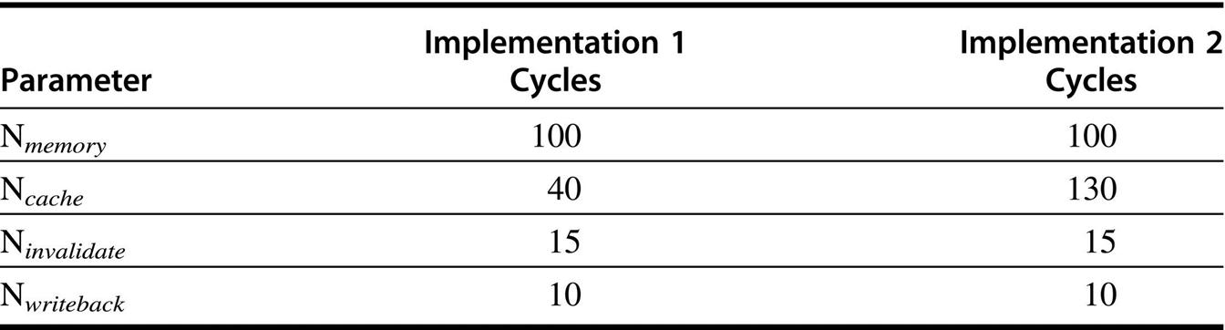
Case Study 2: Simple Directory-Based Coherence
Concepts illustrated by this case study
Consider the distributed shared-memory system illustrated in Figure 5.39. It consists of 8 nodes of processor cores organized as three-dimensional hypercube with point-to-point interconnections, as shown in the figure. For simplification, we assume the following scaled-down configuration:
- Every node has a single processor core with a direct-mapped L1 data cache with its dedicated cache controller.
- The L1 data cache has a capacity of two cache lines with a line size of B bytes.
- The L1 cache states are denoted M, S, and I for Modified, Shared, and Invalid. An example cache entry in some would like
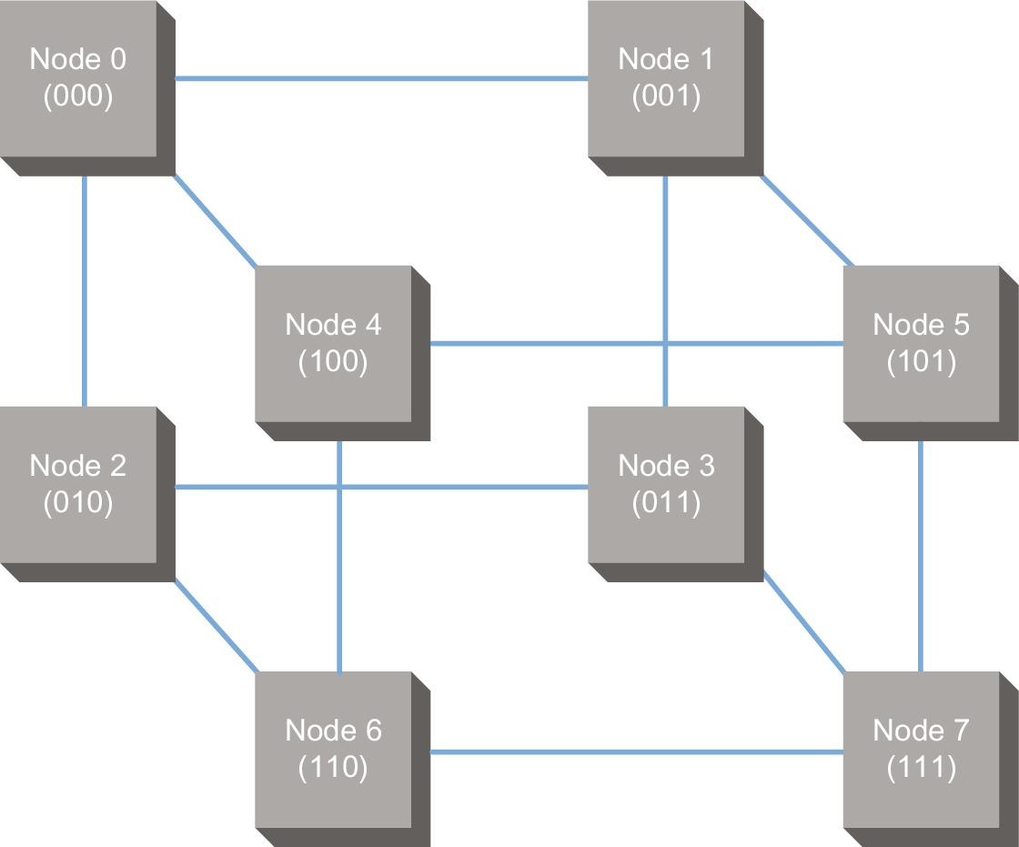
1: S, M3, 0xabcd -->
Cache line 1 is in the “Shared” state; it contains memory block M3 and the data value of the block is 0xabcd.
- The system memory comprises 8 memory blocks (i.e., one memory block per node) and is distributed among the eight nodes, with every node owning a memory block. Node Ci owns memory block Mi.
- Each memory block is B-bytes wide and is tracked by a coherency directory entry stored with the memory block.
- The state of each memory directory entry is denoted DM, DS, and DI for Directory Modified, Directory Shared, and Directory Invalid. Additionally, the directory entry lists the block sharers using a bit vector with 1 bit for every node. Here is an example memory block and associated directory entry:
M3: 0XABCD, DS, 00000011 -->
Memory block M3 (in node C3) contains the value 0xABCD and is shared by nodes 0 and 1 (corresponding to 1s in the bit vector).
Read/Write Notation
To describe read/write transactions, we will use the notation
- C3: R, M2 describes the core in node 3 issuing a read transaction from an address at memory block M2 (the address may possibly be cached in C3 already).
- C0: W, M3 <-- 0018 describes the core in node 0 issuing a write transaction (data is 0X0018) to an address at memory block M3 (the address may possibly be cached in C0 already).
Messages
The directory coherency schemes depend on exchange of command and/or data messages as described by the directory protocol described in Figure 5.20. An example of a command message is a read request. An example of a data message is a read response (with data included).
- Messages originating an ending in the same node do not cross any inter-node links.
- Message with distinct source/destination nodes travel through inter-node links. These messages may be destined from one cache controller to another, from a cache controller to a directory controller, or from a directory controller to a cache controller.
- Messages traveling from a source node to a distinct destination node are statically routed.
- ○ The static routing algorithm selects a shorted path between the source and destination nodes.
- ○ The short path is determined by considering the binary representations of the source and destination indices (e.g., 001 for node C1 and 100 for node C4), then by moving from one node to a neighboring node that was not already crossed by the message.
- – For example, to go from node 6 to node 0 (110 --> 000), the path is 110--> 100--> 000.
- – Because more than one shorted path may exist (110--> 010--> 000 is another path for the preceding example), we assume that the path is selected by inverting first the least significant bit that is different from the corresponding bit in destination index. For example, to travel from node 1 to node 6 (001--> 110), the path is 001--> 000--> 010--> 110.
- ○ The longest possible path traveled by any message has 3 links (equal to the number of bits in the binary representation of a node index).
- A node can simultaneously process up to three messages from/to distinct neighboring nodes' links if no two of them are competing for the same link resource as clarified by the following examples of messages sent/received to/from/through node 000.
Messages: from 001 --> 010; 010 --> 000 (to cache/directory controller); 100 --> 001. OK (distinct destinations).
Message: from 001 --> 010; 000 --> 001 (from cache/directory controller); 100 --> 001.
Not OK as two messages are destined to node 001
In case of destination contention, ties are broken assigning priority to - Assume the transmission and service delays in the following table.
Message type Cache controller Directory controller Link No data 2 cycles 5 cycles 10 cycles With data (  ) cycles
(  ) cycles
(  )
)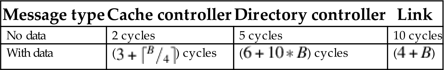
- If a message is forwarded through a node, it is first completely received by the node before being sent to the next node on the path.
- Assume any cache controller; directory controller has unlimited capacity to enqueue messages and service them in FCFS order.
- 5.9. [10/10/10] <5.4> For each part of this exercise, assume that initially all caches lines are invalid, and the data in memory Mi is the byte i (0X00 <= i <= 0x07) repeated as many times as the block size. Assume that successive requests are completely serialized. That is, no core will issue a coherency request until the previous request (by same or different core) is completed.
For each of the following parts, - 5.10. [10/10/10] <5.4> The directory protocol used in 5.9 (based on Figure 5.20) assumes that the directory controller receives requests, sends invalidates, receives modified data, sends modified data to requester if block was dirty, and so on. Assume now that the directory controller will delegate some work to the cores. For example, it will notify the exclusive owner of a modified block when some other core needs the block and will have the owner send the block to the new sharer. Specifically, consider the following optimizations and indicate what their benefits (if any) are. Also, specify how the messages will be modified (in comparison with Figure 5.20 protocol) to support the new change.
Hint: Benefits might be reduction in number of messages, faster response time, and so on.- a. [10] <5.4> On a write miss to a shared memory block, the directory controller sends the data to the requester and instructs the sharers to send their invalidate acknowledgements directly to the requester.
- b. [10] <5.4> On a read miss to a block modified in some other core, the directory controller instructs the owner of the modified copy to directly forward the data to the requester.
- c. [10] <5.4> On a read miss to a block in shared (S) state in some other cores, the directory controller instructs one of the sharers (say, the one closest to the requester) to directly forward the data to the requester.
- 5.11. [15/15/15] <5.4> In problem 5.9, it was assumed that all transactions on the system were serially executed, which is both unrealistic and inefficient in a DSM multicore. We now relax this condition. We will require only that all transactions originating in one core are serialized. However, different cores can independently issue their read/write transactions and even compete for the same memory block. The transactions of problem 5.9 are represented next to reflect the new, relaxed constraints. Redo problem 5.9 with the new, relaxed constraints.
- 5.12. [10/10] <5.4> Use the routing and delay information described earlier and trace how the following groups of transactions will progress in the system (assume that all accesses are misses).
- 5.13. [20] <5.4> What extra complexities may arise if the messages can be adaptively rerouted on the links? For example, a coherency message from core M1 directory controller to C2 (expressed in binary as M001 --> C010) will be routed either through the inter-node path C001--> C000--> C010 or the inter-node path C001--> C011--> C010, depending on link availability.
- 5.14. [20] <5.4> In a read miss, a cache might overwrite a line in the shared (S) state without notifying the directory that owns the corresponding memory block. Alternatively, it will notify the directory so that it deletes this cache from the list of sharers.
Show how the following transaction groups (performed one at a time in series) will proceed under both approaches.
 C3: R, M4
 C3: R, M2
 C2: W, M4 <--0xabcd
Case Study 3: Memory Consistency
Concepts Illustrated by This Case Study
- 5.15. [10/10] <5.6> Consider the following code segments running on two processors P1 and P2. Assume A and B are initially 0.
P1: P2: While (B == 0); While (A==0); A=1; B = 1; - 5.16. [5] <5.6> Consider the following code segments running on two processors P1 and P2. Assume A, and B, are initially 0. Explain how an optimizing compiler might make it impossible for B to be ever set to 2 in a sequentially consistent execution model.
P1: P2: A=1; B=1; A=2; While (A <> 1); While (B == 0); B = 2; - 5.17. [10] <5.4>. In a processor implementing a SC consistency model, the data cache is augmented with a data prefetch unit. Will that alter the SC implementation execution results? Why or why not?
- 5.18. [10/10] <5.6> Assume that the following code segment is executed on a processor that implements partial store order (PSO),
 A=1;
 B=2;
 If (C== 3)
 D=B;
- 5.19. [20/20/20] <5.6> Sequential consistency (SC) requires that all reads and writes appear to have executed in some total order. This may require the processor to stall in certain cases before committing a read or write instruction. Consider the code sequence
write A
read B
where the write A results in a cache miss and the read B results in a cache hit.
Under SC, the processor must stall read B until after it can order (and thus perform) write A. Simple implementations of SC will stall the processor until the cache receives the data and can perform the write.
Release consistency (RC) consistency mode (see Section 5.6) relaxes these constraints: ordering—when desired—is enforced by judicious use of synchronization operations. This allows, among other optimizations, processors to implement write buffers, which hold committed writes that have not yet been ordered with respect to other processors' writes. Reads can pass (and potentially bypass) the write buffer in RC (which they could not do in SC).
Assume that one memory operation can be performed per cycle and that operations that hit in the cache or that can be satisfied by the write buffer introduce no stall cycles. Operations that miss incur the latencies listed in Figure 5.38.
How many stall cycles occur prior to each operation for both the SC and RC consistency models? (Write buffer can hold at most one write.)- a. [20] <5.6> P0: write 110 <-- 80 //assume miss (no other cache has the line)
- P0: read 108 //assume miss (no other cache has the line)
- b. [20] <5.6> P0: read 110 //assume miss (no other cache has the line)
- P0: write 100 <-- 90 //assume hit
- c. [20] <5.6> P0: write 100 <-- 80 //assume miss
- P0: write 110 <-- 90 //assume hit
- 5.20. [20] <5.6> Repeat part (a) of problem 5.19 under an SC model on a processor that has a read prefetch unit. Assume a read prefetch was triggered 20 cycles in advance of the write operation.
Exercises
- 5.21. [15] <5.1> Assume that we have a function for an application of the form F(i, p), which gives the fraction of time that exactly i processors are usable given that a total of p processors are available. This means that
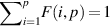
Assume that when i processors are in use, the applications run i times faster.- a. Rewrite Amdahl's Law so that it gives the speedup as a function of p for some application.
- b. An application A runs on single processor for a time T seconds. Different portions of its running time can improve if a larger number of processors is used. Figure 5.40 provides the details.
How much speedup will A achieve when on 8 processors? - c. Repeat for 32 processors and an infinite number of processors.
- 5.22. [15/20/10] <5.1> In this exercise, we examine the effect of the interconnection network topology on the CPI of programs running on a 64-processor distributed-memory multiprocessor. The processor clock rate is 2.0 GHz, and the base CPI of an application with all references hitting in the cache is 0.75. Assume that 0.2% of the instructions involve a remote communication reference. The cost of a remote communication reference is (100 + 10 h) ns, h being the number of communication network hops that a remote reference has to make to the remote processor memory and back. Assume all communication links are bidirectional.
- a. [15] <5.1> Calculate the worst-case remote communication cost when the 64 processors are arranged as a ring, as an 8 × 8 processor grid, or as a hypercube (hint: longest communication path on a 2n hypercube has n links).
- b. [20] <5.1> Compare the base CPI of the application with no remote communication to the CPI achieved with each of the three topologies in part (a).
- 5.23. [15] <5.2> Show how the basic snooping protocol of Figure 5.6 can be changed for a write-through cache. What is the major hardware functionality that is not needed with a write-through cache compared with a write-back cache?
- 5.24. [20/20] <5.2> Please answer the following problems:
- a. [20] <5.2> Add a clean exclusive state to the basic snooping cache coherence protocol (Figure 5.6). Show the protocol in the finite state machine format used in the figure.
- b. [20] <5.2> Add an “owned” state to the protocol of part (a) and describe using the same finite state machine format used in Figure 5.6.
- 5.25. [15] <5.2> One proposed solution for the problem of false sharing is to add a valid bit per word. This would allow the protocol to invalidate a word without removing the entire block, letting a processor keep a portion of a block in its cache while another processor writes a different portion of the block. What extra complications are introduced into the basic snooping cache coherence protocol (Figure 5.6) by this addition? Consider all possible protocol actions.
- 5.26. [15/20] <5.3> This exercise studies the impact of aggressive techniques to exploit instruction-level parallelism in the processor when used in the design of shared-memory multiprocessor systems. Consider two systems identical except for the processor. System A uses a processor with a simple single-issue, in-order pipeline, and system B uses a processor with four-way issue, out-of-order execution and a reorder buffer with 64 entries.
- a. [15] <5.3> Following the convention of Figure 5.11, let us divide the execution time into instruction execution, cache access, memory access, and other stalls. How would you expect each of these components to differ between system A and system B?
- b. [10] <5.3> Based on the discussion of the behavior of OLTP workload in Section 5.3, what is the important difference between the OLTP workload and other benchmarks that limit benefit from a more aggressive processor design?
- 5.27. [15] <5.3> How would you change the code of an application to avoid false sharing? What might be done by a compiler and what might require programmer directives?
- 5.28. [15] <5.3> An application is calculating the number of occurrences of a certain word in a very large number of documents. A very large number of processors divided the work, searching the different documents. They created a huge array—word_count—of 32-bit integers, every element of which is the number of times the word occurred in some document. In a second phase, the computation is moved to a small SMP server with four processors. Each processor sums up approximately ¼ of the array elements. Later, one processor calculates the total sum.
for (int p = 0; p<=3; p++) // Each iteration of is executed on a separate processor. { sum [p] = 0; for (int i = 0; i < n/4; i++) // n is size of word_count and is divisible by 4 sum[p] = sum[p] + word_count[p+4*i]; } total_sum = sum[0] + sum[1]+sum[2]+sum[3] //executed only on processor. - 5.29. [15] <5.4> Assume a directory-based cache coherence protocol. The directory currently has information that indicates that processor P1 has the data in “exclusive” mode. If the directory now gets a request for the same cache block from processor P1, what could this mean? What should the directory controller do? (Such cases are called “race conditions” and are the reason why coherence protocols are so hard to design and verify.)
- 5.30. [20] <5.4> A directory controller can send invalidates for lines that have been replaced by the local cache controller. To avoid such messages, and to keep the directory consistent, replacement hints are used. Such messages tell the controller that a block has been replaced. Modify the directory coherence protocol of Section 5.4 to use such replacement hints.
- 5.31. [20/15/20/15] <5.4> One downside of a straightforward implementation of directories using fully populated bit vectors is that the total size of the directory information scales as the product: processor count × memory blocks. If memory grows linearly with processor count, the total size of the directory grows quadratically in the processor count. In practice, because the directory needs only 1 bit per memory block (which is typically 32–128 bytes), this problem is not serious for small-to-moderate processor counts. For example, assuming a 128-byte block, and P processors, the amount of directory storage compared to main memory is P/(128*8) = P/1024, which is 12.5% overhead for P = 128 processors. We can avoid this problem by observing that we need to keep only an amount of information that is proportional to the cache size of each processor. We explore some solutions in these exercises.
- a. [20] <5.4> One method to obtain a scalable directory protocol is to organize the multiprocessor as a logical hierarchy with the processors as leaves of the hierarchy and directories positioned at the root of each subtree. The directory at each subtree records which descendants cache which memory blocks. It also records the memory blocks—with a home in that subtree—that are cached outside the subtree. Compute the amount of storage needed to record the processor information for the directories, assuming that each directory is fully associative. Your answer should incorporate both the number of nodes at each level of the hierarchy as well as the total number of nodes.
- b. [15] <5.4> Another approach to reducing the directory size is to allow only a limited number of the directory's memory blocks to be shared at any given time. Implement the directory as a four-way set-associative cache storing full bit vectors. If a directory cache miss occurs, choose a directory entry and invalidate the entry. Describe how this organization will work elaborating what will happen as a is block read, written replaced and written back to memory. Modify the protocol in Figure 5.20 to reflect the new transitions required by this directory organization.
- c. [20] <5.4> Rather than reducing the number of directory entries, we can implement bit vectors that are not dense. For example, we can set every directory entry to 9 bits. If a block is cached in only one node outside its home, this field contains the node number. If the block is cached in more than one node outside its home, this field is a bit vector with each bit indicating a group of eight processors, at least one of which caches the block. Illustrate how this scheme would work for a 64-processor DSM machine that consists of eight 8-processors groups.
- d. [15] An extreme approach to reducing the directory size is to implement an “empty” directory; that is, the directory in every processor does not store any memory states. It receives requests and forwards them as appropriate. What is the benefit of having such a directory over having no directory at all for a DSM system?
- 5.32. [10] <5.5> Implement the classical compare-and-swap instruction using the load linked/store conditional instruction pair.
- 5.33. [15] <5.5> One performance optimization commonly used is to pad synchronization variables so as not to have any other useful data in the same cache line. Construct an example demonstrating that this optimization can be extremely useful in some situations. Assume a snoopy write invalidate protocol.
- 5.34. [30] <5.5> One possible implementation of the load linked/store conditional pair for multicore processors is to constrain these instructions to using uncached memory operations. A monitor unit intercepts all reads and writes from any core to the memory. It keeps track of the source of the load linked instructions and whether any intervening stores occur between the load linked and its corresponding store conditional instruction. The monitor can prevent any failing store conditional from writing any data and can use the interconnect signals to inform the processor that this store failed.
Design such a monitor for a memory system supporting a four-core SMP. Take into account that, generally, read and write requests can have different data sizes (4/8/16/32 bytes). Any memory location can be the target of a load linked/store conditional pair, and the memory monitor should assume that load linked/store conditional references to any location can, possibly, be interleaved with regular accesses to the same location. The monitor complexity should be independent of the memory size. - 5.35. [25] <5.5> Prove that, in a two-level cache hierarchy where L1 is closer to the processor, inclusion is maintained with no extra action if L2 has at least as much associativity as L1, both caches use LRU replacement, and both caches have the same block sizes.
- 5.36. [Discussion] <5> When trying to perform detailed performance evaluation of a multiprocessor system, system designers use one of three tools: analytical models, trace-driven simulation, and execution-driven simulation. Analytical models use mathematical expressions to model the behavior of programs. Trace-driven simulations run the applications on a real machine and generate a trace, typically of memory operations. These traces can be replayed through a cache simulator or a simulator with a simple processor model to predict the performance of the system when various parameters are changed. Execution-driven simulators simulate the entire execution maintaining an equivalent structure for the processor state and so on.
- a. What are the accuracy/speed trade-offs between these approaches?
- b. CPU traces, if not carefully collected, can exhibit artifacts of the system they are collected on. Discuss this issue while using branch-prediction and spin-wait synchronization as examples. (Hint: The program itself is not available to a pure CPU trace; just the trace is available.)
- 5.37. [40] <5.7, 5.9> Multiprocessors and clusters usually show performance increases as you increase the number of the processors, with the ideal being n times speedup for n processors. The goal of this biased benchmark is to make a program that gets worse performance as you add processors. For example, this means that one processor on the multiprocessor or cluster runs the program fastest, two are slower, four are slower than two, and so on. What are the key performance characteristics for each organization that give inverse linear speedup?