
SENSORS TURN REAL-WORLD measurements into electronic signals that we can then use on our Arduino boards. The projects in this chapter are all about using light and temperature.
We also look at how to interface with keypads and rotary encoders.
This project would not be out of place in the lair of any Evil Genius worth their salt. A secret code must be entered on the keypad, and if it is correct, a green LED will light; otherwise, a red LED will stay lit. In Project 27 we will revisit this project and show how it cannot just show the appropriate light but also control a door lock.
COMPONENTS AND EQUIPMENT
Unfortunately, keypads do not usually have pins attached, so we will have to attach some, and the only way to do that is to solder them on. So this is another of our projects where you will have to do a little soldering.
The schematic diagram for Project 10 is shown in Figure 5-1. By now, you will be used to LEDs; the new component is the keypad.

Figure 5-1 Schematic diagram for Project 10.
Keypads are normally arranged in a grid so that when one of the keys is pressed, it connects a row to a column. Figure 5-2 shows a typical arrangement for a 12-key keypad with numbers from 0 to 9 and * and # keys.

Figure 5-2 A 12-key keypad.
The key switches are arranged at the intersection of row-and-column wires. When a key is pressed, it connects a particular row to a particular column.
By arranging the keys in a grid like this, it means that we only need to use 7 (4 rows + 3 columns) of our digital pins rather than 12 (one for each key).
However, it also means that we have to do a bit more work in the software to determine which keys are pressed. The basic approach we have to take is to connect each row to a digital output and each column to a digital input. We then put each output high in turn and see which inputs are high.
Figure 5-3 shows how you can solder seven pins from a pin header strip onto the keypad so that you can then connect it to the breadboard. Pin headers are bought in strips and can be easily snapped to provide the number of pins required.

Figure 5-3 Soldering pins to the keypad.
Now we just need to find out which pin on the keypad corresponds to which row or column. If we are lucky, the keypad will come with a datasheet that tells us this. If not, we will have to do some detective work with a multimeter. Set the multimeter to continuity so that it beeps when you connect the leads together. Then get some paper, draw a diagram of the keypad connections, and label each pin with a letter from a to g. Then write a list of all the keys. Then, holding each key down in turn, find the pair of pins that make the multimeter beep, indicating a connection (Figure 5-4). Release the key to check that you have indeed found the correct pair. After a while, a pattern will emerge, and you will be able to see how the pins relate to rows and columns. Figure 5-4 shows the arrangement for the keypad used by the author.

Figure 5-4 Working out the keypad connections.
The completed breadboard layout is shown in Figure 5-5 and the assembled breadboard in Figure 5-6. Note that your keypad may have a different pinout. If so, you will need to change the jumper wires connected to it accordingly.

Figure 5-5 Project 10 breadboard layout.
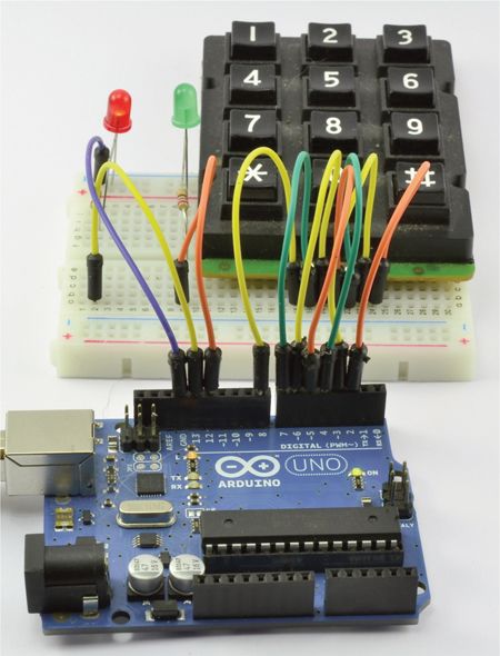
Figure 5-6 Project 10 keypad security code.
You may have noticed that digital pins 0 and 1 have “TX” and “RX” next to them. This is so because they are also used by the Arduino board for serial communications, including the USB connection. It is common to avoid using these pins for general-purpose input-output duties so that serial communications, including programming the Arduino, can take place without the need to disconnect any wires.
While we could just write a sketch that turns on the output for each row in turn and reads the inputs to get the coordinates of any key pressed, it is a bit more complex than that because switches do not always behave in a good way when you press them. Keypads and push switches are likely to bounce. That is, when you press them, they do not simply go from being opened to closed but may open and close several times as part of pressing the button.
Fortunately for us, Mark Stanley and Alexander Brevig have created a library that you can use to connect to keypads that handle such things for us. This is a good opportunity to demonstrate installing a library into the Arduino software.
In addition to the libraries that come with the Arduino, many people have developed their own libraries and published them for the benefit of the Arduino community. The Evil Genius is much amused by such altruism and sees it as a great weakness. However, the Evil Genius is not above using such libraries for his own devious ends.
To make use of this library, we must first download it from the Arduino website at this address: www.arduino.cc/playground/Code/Keypad.
Download the file Keypad.zip to your desktop.
Whether using Windows, Mac, or LINUX, you will find that the Arduino software has created a folder in your “Documents” folder that contains a directory called “Arduino.” Libraries that you download all should be installed in a folder called “Libraies” within this “Arduino” directory. If this is the first library you have installed, you will need to create this folder.
Figure 5-7 shows how you can create this folder as you extract the “Library” folder from the Zip file

Figure 5-7 Unzipping the library for Windows.
Once you have installed this library into your “Arduino” directory, you will be able to use it with any sketches that you write.
You can check that the library is installed correctly by restarting the Arduino IDE and selecting the “Examples” option from the File menu. You should now find that there is a new category for the “Keypad” library (Figure 5-8).
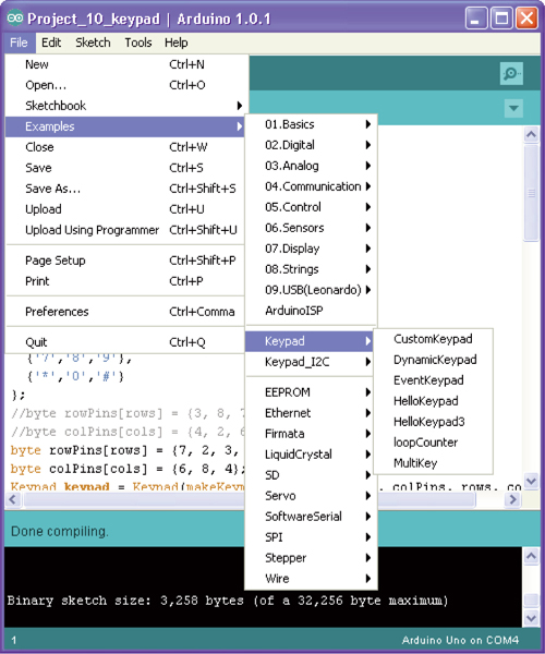
Figure 5-8 Checking the installation.
The sketch for the application is shown in Listing Project 10. Note that you may well have to change your keys’ rowPins and colPins arrays so that they agree with the key layout of your keypad, as we discussed in the hardware section.
LISTING PROJECT 10


This sketch is quite straightforward. The loop function checks for a key press. If the key pressed is a # or a *, it sets the position variable back to 0. If, on the other hand, the key pressed is one of the numerals, it checks to see if the next key expected (secretCode[position]) is the key just pressed, and if it is, it increments position by one. Finally, the loop checks to see if position is 4, and if it is, it sets the LEDs to their unlocked state.
Load the completed sketch for Project 10 from your Arduino Sketchbook and download it to the board (see Chapter 1).
If you have trouble getting this to work, it is most likely a problem with the pin layout on your keypad. So persevere with the multimeter to map out the pin connections.
We have already met variable resistors: As you turn the knob, the resistance changes. These used to be behind most knobs that you could twiddle on electronic equipment. There is an alternative, the rotary encoder, and if you own some consumer electronics where you can turn the knob round and round indefinitely without meeting any kind of end stop, there is probably a rotary encoder behind the knob.
Some rotary encoders also incorporate a button so that you can turn the knob and then press. This is a particularly useful way of making a selection from a menu when used with a liquid-crystal display (LCD) screen.
A rotary encoder is a digital device that has two outputs (A and B), and as you turn the knob, you get a change in the outputs that can tell you whether the knob has been turned clockwise or counterclockwise.
Figure 5-9 shows how the signals change on A and B when the encoder is turned. When rotating clockwise, the pulses will change, as they would moving left to right on the diagram; when moving counterclockwise, the pulses would be moving right to left on the diagram.

Figure 5-9 Pulses from a rotary encoder.
So, if A is low and B is low and then B becomes high (going from phase 1 to phase 2), that would indicate that we have turned the knob clockwise. A clockwise turn also would be indicated by A being low, B being high, and then A becoming high (going from phase 2 to phase 3), etc. However, if A were high and B were low and then B went high, we have moved from phase 4 to phase 3 and are therefore turning counterclockwise.
This project uses a rotary encoder with a built-in push switch to control the sequence of the traffic signals and is based on Project 5. It is a much more realistic version of a traffic signal controller and is really not far off the logic that you would find in a real traffic signal controller.
Rotating the rotary encoder will change the frequency of the light sequencing. Pressing the button will test the lights, turning them all on at the same time, while the button is pressed.
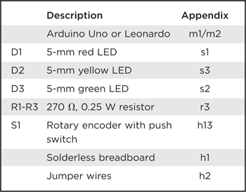
The components are the same as for Project 5, with the addition of the rotary encoder in place of the original push switch.
COMPONENTS AND EQUIPMENT
The schematic diagram for Project 11 is shown in Figure 5-10. The majority of the circuitry is the same as for Project 5, except that now we have a rotary encoder.

Figure 5-10 Schematic diagram for Project 11.
The rotary encoder works just as if there were three switches: one each for A and B and one for the push switch.
Since the schematic is much the same as for Project 5, it will not be much of a surprise to see that the breadboard layout (Figure 5-11) is also similar to the one for that project.

Figure 5-11 Breadboard layout for Project 11.
The starting point for the sketch is the sketch for Project 5. We have added code to read the encoder and to respond to the button press by turning all the LEDs on. We also have taken the opportunity to enhance the logic behind the lights to make them behave in a more realistic way, changing automatically. In Project 5, when you held down the button, the lights changed sequence roughly once per second. In a real traffic signal, the lights stay green and red a lot longer than they are yellow. So our sketch now has two periods: shortPeriod, which does not alter but is used when the lights are changing, and longPeriod, which determines how long they are illuminated when green or red. This longPeriod is the period that is changed by turning the rotary encoder.
The key to handling the rotary encoder lies in the function getEncoderTurn. Every time this is called, it compares the previous state of A and B with their current state, and if something has changed, it works out whether it was clockwise or counterclockwise and returns a -1 or 1, respectively. If there is no change (the knob has not been turned), it returns 0. This function must be called frequently, or turning the rotary controller quickly will result in some changes not being recognized correctly.
If you want to use a rotary encoder for other projects, you can just copy this function. The function uses the static modifier for the oldA and oldB variables. This is a useful technique that allows the function to retain the values between one call of the function and the next, where normally it would reset the value of the variable every time the function is called.
LISTING PROJECT 11

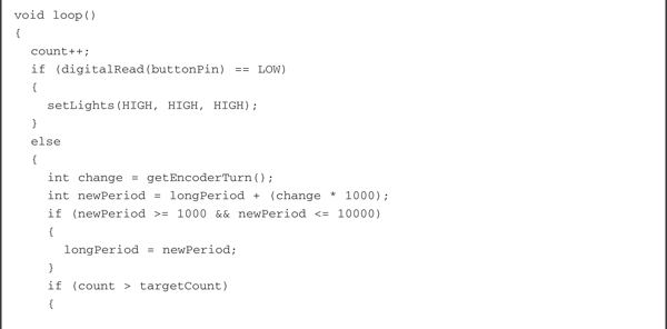


This sketch illustrates a useful technique that lets you time events (turning an LED on for so many seconds) while at the same time checking the rotary encoder and button to see if they have been turned or pressed. If we just used the Arduino delay function with, say, 20,000, for 20 seconds, we would not be able to check the rotary encoder or switch in that period.
So what we do is use a very short delay (1 millisecond) but maintain a count that is incremented each time round the loop. Thus, if we want to delay for 20 seconds, we stop when the count has reached 20,000. This is less accurate than a single call to the delay function because the 1 millisecond is actually 1 millisecond plus the processing time for the other things that are done inside the loop.
Load the completed sketch for Project 11 from your Arduino Sketchbook and download it to the board (see Chapter 1).
You can press the rotary encoder button to test the LEDs and turn the rotary encoder to change how long the signal stays green and red.
A common and easy-to-use device for measuring light intensity is the light-dependent resistor (or LDR). They are also sometimes called photoresistors.
The brighter the light falling on the surface of the LDR, the lower is the resistance. A typical LDR will have a dark resistance of up to 2 MΩ and a resistance when illuminated in bright daylight of perhaps 20 kΩ.
We can convert this change in resistance to a change in voltage by using the LDR, with a fixed resistor as a voltage divider, connected to one of our analog inputs. The schematic for this is shown in Figure 5-12.

Figure 5-12 Using an LDR to measure light.
With a fixed resistor of 100K, we can do some rough calculations about the voltage range to expect at the analog input.
In darkness, the LDR will have a resistance of 2 MΩ, so with a fixed resistor of 100K, there will be about a 20:1 ratio of voltage, with most of that voltage across the LDR, so this would mean about 4V across the LDR and 1V at the analog pin.
On the other hand, if the LDR is in bright light, its resistance might fall to 20 kΩ. The ratio of voltages then would be about 4:1 in favor of the fixed resistor, giving a voltage at the analog input of about 4V.
A more sensitive photo detector is the phototransistor. This functions like an ordinary transistor except there is not usually a base connection. Instead, the collector current is controlled by the amount of light falling on the phototransistor.
This project uses an ultrabright infrared (IR) LED and a phototransistor to detect the pulse in your finger. It then flashes a red LED in time with your pulse.
COMPONENTS AND EQUIPMENT

The pulse monitor works as follows: Shine the bright LED onto one side of your finger while the phototransistor on the other side of your finger picks up the amount of transmitted light. The resistance of the phototransistor will vary slightly as the blood pulses through your finger.
The schematic for this is shown in Figure 5-13 and the breadboard layout in Figure 5-15. We have chosen quite a high value of resistance for R1 because most of the light passing through the finger will be absorbed, and we want the phototransistor to be quite sensitive. You may need to experiment with the value of the resistor to get the best results.

Figure 5-13 Schematic for Project 12.
It is important to shield the phototransistor from as much stray light as possible. This is particularly important for domestic lights that actually fluctuate at 50 or 60 Hz and will add a considerable amount of noise to our weak heart signal.
For this reason, the phototransistor and LED are built into a tube or corrugated cardboard held together with duct tape. The construction of this is shown in Figure 5-14.

Figure 5-14 Sensor tube for heart monitor.
Two 5-mm holes are drilled opposite each other in the tube, and the LED is inserted into one side and the phototransistor into the other. Short leads are soldered to the LED and phototransistor, and then another layer of tape is wrapped over everything to hold it all in place. Be sure to check which colored wire is connected to which lead of the LED and phototransistor before you tape them up.
It is also a good idea to use screened wire for the phototransistor to reduce interference. It is also worth noting that a peculiarity of most IR LEDs is that the longer lead is negative rather than positive, so check the data sheet of the device before you attach it.
The breadboard layout for this project (Figure 5-15) is very straightforward.
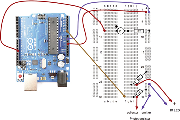
Figure 5-15 Breadboard layout for Project 12.
The final “finger tube” can be seen in Figure 5-16.

Figure 5-16 Project 12: pulse-rate monitor.
The software for this project is quite tricky to get right. Indeed, the first step is not to run the entire final script but rather a test script that will gather data that we can then paste into a spreadsheet and chart to test out the smoothing algorithm (more on this later).
The test script is provided in Listing Project 12.
LISTING PROJECT 12—TEST SCRIPT

This script reads the raw signal from the analog input, applies the smoothing function, and then writes both values to the Serial Monitor, where we can capture them and paste them into a spreadsheet for analysis. Note that the Serial Monitor’s communications is set to its fastest rate to minimize the effects of the delays caused by sending the data. When you start the Serial Monitor, you will need to change the serial speed to 115,200 baud.
The smoothing function uses a technique called leaky integration, and you can see in the code where we do this smoothing using the line

The variable alpha is a number greater than 0 but less than 1 and determines how much smoothing to do.
Put your finger into the sensor tube, start the Serial Monitor, and leave it running for 3 or 4 seconds to capture a few pulses.
Then copy and paste the captured text into a spreadsheet. You will probably be asked for the column delimiter character, which is a comma. The resulting data and a line chart drawn from the two columns are shown in Figure 5-17.

Figure 5-17 Heart monitor test data pasted into a spreadsheet.
The more jagged trace is from the raw data read from the analog port, and the smoother trace clearly has most of the noise removed. If the smoothed trace shows significant noise—in particular, any false peaks that will confuse the monitor—increase the level of smoothing by decreasing the value of alpha.
Once you have found the right value of alpha for your sensor arrangement, you can transfer this value into the real sketch and switch over to using the real sketch rather than the test sketch. The real sketch is provided in the following listing.
LISTING PROJECT 12

There now just remains the problem of detecting the peaks. Looking at Figure 5-17, we can see that if we keep track of the previous reading, we can see that the readings are gradually increasing until the change in reading flips over and becomes negative. So, if we lit the LED whenever the old change was positive but the new change was negative, we would get a brief pulse from the LED at the peak of each pulse.
Both the test and real sketch for Project 12 are in your Arduino Sketchbook. For instructions on downloading it to the board, see Chapter 1.
As mentioned earlier, getting this project to work is a little tricky. You will probably find that you have to get your finger in just the right place to start getting a pulse. If you are having trouble, run the test script as described previously to check that your detector is getting a pulse and the smoothing factor alpha is low enough.
The author would like to point out that this device should not be used for any kind of real medical application.
Measuring temperature is a similar problem to measuring light intensity. Instead of an LDR, a device called a thermistor is used. As the temperature increases, so does the resistance of the thermistor.
When you buy a thermistor, it will have a stated resistance. In this case, the thermistor chosen is 33 kΩ. This will be the resistance of the device at 25°C.
The formula for calculating the resistance at a particular temperature is given by
R = Ro exp(-beta/(T + 273) - beta/(To + 273)
You can do the math if you like, but a much simpler way to measure temperature is to use a special-purpose thermometer chip such as the TMP36. This three-pinned device has two pins for the power supply (5V) and a third output pin, whose temperature T in degrees C is related to the output voltage V by the equation
T = (V - 0.5) × 100
So, if the voltage at its output is 1V, the temperature is 50°C.
This project is controlled by your computer, but once given its logging instructions, the device can be disconnected and run on batteries to do its logging. While logging, it stores its data, and then when the logger is reconnected, it will transfer its data back over the USB connection, where it can be imported into a spreadsheet. By default, the logger will record one sample every 5 minutes and can record up to 1000 samples.
To instruct the temperature logger from your computer, we have to define some commands that can be issued from the computer. These are shown in Table 5-1.
TABLE 5-1 Temperature Logger Commands

This project just requires a TMP36 that can fit directly into the sockets on the Arduino.
COMPONENTS AND EQUIPMENT

The schematic diagram for Project 13 is shown in Figure 5-18.

Figure 5-18 Schematic diagram for Project 13.
This is so simple that we can simply fit the leads of the TMP36 into the Arduino board, as shown in Figure 5-19. Note that the curved side of the TMP36 should face outward from the Arduino. Putting a little kink in the leads with pliers will ensure a better contact.

Figure 5-19 Project 13: temperature logger.
Two of the analog pins (A0 and A2) are going to be used for the GND and 5V power connections to the TMP36. The TMP36 uses very little current, so the pins can easily supply enough to power it if we set one pin HIGH and the other LOW.
The software for this project is a little more complex than for some of our other projects (see Listing Project 13). All the variables that we have used in our sketches so far are forgotten as soon as the Arduino board is reset or disconnected from the power. Sometimes we want to be able to store data persistently so that it is there next time we start up the board. This can be done by using the special type of memory on the Arduino called EEPROM, which stands for electrically erasable programmable read-only memory. The Arduino Uno and Leonardo both have 1024 bytes of EEPROM.
For the data logger to be useful, it needs to remember the readings that it has already taken, even when it is disconnected from the computer and powered from a battery. It also needs to remember the logging period.
This is the first project where we have used the Arduino’s EEPROM to store values so that they are not lost if the board is reset or disconnected from the power. This means that once we have set our data-logging recording, we can disconnect it from the USB lead and leave it running on batteries. Even if the batteries go dead, our data will still be there the next time we connect it.


You will notice that at the top of this sketch we use the command #define for what in the past we would have used variables for. This is actually a more efficient way of defining constants—that is, values that will not change during the running of the sketch. So it is actually ideal for pin settings and constants such as beta. The command #define is what is called a preprocessor directive, and what happens is that just before the sketch is compiled, all occurrences of its name anywhere in the sketch are replaced by its value. It is very much a matter of personal taste whether you use #define or a variable.
Fortunately, reading and writing EEPROM happens just 1 byte at a time. So, if we want to write a variable that is a byte or a char, we can just use the functions EEPROM.write and EEPROM.read, as shown in the example here:

The 0 in the parameters for read and write is the address in the EEPROM to use. This can be any number between 0 and 1023, with each address being a location where 1 byte is stored.
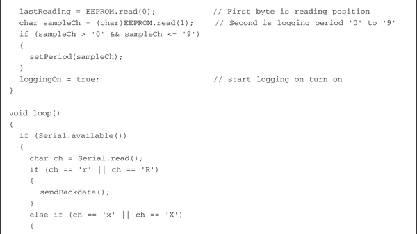
In this project we want to store both the position of the last reading taken (in the lastReading variable) and all the readings. So we will record lastReading in the first byte of EEPROM, the logging period as a character 1 to 9, and then the actual reading data in the bytes that follow.
Each temperature reading is kept in a float, and if you remember from Chapter 2, a float occupies 4 bytes of data. Here we had a choice: We could either store all 4 bytes or find a way to encode the temperature into a single byte. We decided to take the latter route so that we can store as many readings as possible in the EEPROM.
The way we encode the temperature into a single byte is to make some assumptions about our temperatures. First, we assume that any temperature in Centigrade will be between –20 and +40. Anything higher or lower would likely damage our Arduino board anyway. Second, we assume that we only need to know the temperature to the nearest quarter of a degree.
With these two assumptions, we can take any temperature value we get from the analog input, add 20 to it, multiply it by 4, and still be sure that we always have a number between 0 and 240. Since a byte can hold a number between 0 and 255, that just fits nicely.
When we take our numbers out of EEPROM, we need to convert them back to a float, which we can do by reversing the process, dividing by 4, and then subtracting 20.
Both encoding and decoding the values are wrapped up in the functions storeReading and getReading. So, if we decided to take a different approach to storing the data, we would only have to change these two functions.
Load the completed sketch for Project 13 from your Arduino Sketchbook and download it to the board (see Chapter 1).
Now open the Serial Monitor (Figure 5-20), and for test purposes, we will set the temperature logger to log every minute by typing 1 in the Serial Monitor. The board should respond with the message “Sample period set to: 1 min.” If we wanted to, we could then change the mode to Fahrenheit by typing F into the Serial Monitor. Now we can check the status of the logger by typing? (Figure 5-21).

Figure 5-20 Issuing commands through the Serial Monitor.

Figure 5-21 Displaying the Temperature Logger Status.
In order to unplug the USB cable, we need to have an alternative source of power, such as the battery lead we made back in Project 6. You need to have this plugged in and powered up at the same time as the USB connector is connected if you want the logger to keep logging after you disconnect the USB lead.
Finally, we can type the G command to start logging. We can then unplug the USB lead and leave our logger running on batteries. After waiting 10 or 15 minutes, we can plug it back in to see what data we have by opening the Serial Monitor and typing the R command, the results of which are shown in Figure 5-22. Select all the data, including the “Time” and “Temp” headings at the top.

Figure 5-22 Data to copy and paste into a spreadsheet.
Copy the text to the clipboard (press CTRL-C on Windows and LINUX, ALT-C on Macs), open a spreadsheet in a program such as Microsoft Excel, and paste it into a new spreadsheet (Figure 5-23).

Figure 5-23 Temperature data imported into a spreadsheet.
Once in the spreadsheet, we can even draw a chart using our data.
We now know how to handle various types of sensors and input devices to go with our knowledge of LEDs. In the next section we will look at a number of projects that use light in various ways and get our hands on some more advanced display technologies, such as LCD text panels and seven-segment LEDs.