7.9   THE METHOD OF ITERATION FOR DOMINANT EIGENVALUES

In this section we shall present a method for computing the dominant eigenvalue or eigenvalues of an n × n matrix A. To take the most useful case, we shall assume that A is real. In scientific and engineering applications, we are typically interested in finding the real and the complex eigenvalues of a real matrix. Our analysis could readily be extended to matrices with complex components. In Section 7.10 we will show how to compute the smaller eigenvalues.

A real matrix A has a characteristic polynomial det (λI − A) with real coefficients. Therefore, the eigenvalues of A occur as real numbers or as complex-conjugate pairs, λ and . For clarity, we shall suppose that the eigenvalues λ₁, λ₂, . . . , λ_n of A are distinct, so that A has n linearly independent eigenvectors u¹, u², . . . , uⁿ. (Without difficulty the reader will be able to generalize this analysis, using either the Jordan form of A or an expansion in principal vectors, as in Section 7.6.)

Let . The dominant eigenvalues are defined to be the eigenvalues ot greatest absolute value. We shall consider only two cases.

Real case. Here we suppose that A has a single real eigenvalue λ₁ of maximum absolute value. We allow λ₁ to be either positive or negative. Thus,

 

Complex case. Here we suppose that A has the complex-conjugate dominant eigenvalues

 

Other cases are possible but unusual, and we ignore them. For example, A could have the dominant eigenvalues +1 and −1. Or A could have the five dominant eigenvalues λ_k = −7 exp (2kπi/5) (k = 1, . . . , 5). Observe that, in both of these examples, the translation λ_k → λ_k + 1, caused by adding 1 to each diagonal element of A, produces eigenvalues λ_k + 1 which fall into the real case (1), or the complex case (2).

In the real case (1), we pick an initial vector x⁰ and form the iterates x¹ = Ax⁰, x² = Ax¹, . . . . If x⁰ has the expansion

 

then the iterate x^k has the expansion

 

 

where, since for all .

 

We suppose that ξ₁ ≠ 0. This supposition is almost surely correct if x⁰ is picked in some bizarre way, e.g.,

 

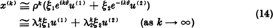
Then for large k, as (5) shows,

 

For large k, successive vectors are approximately multiples of each other, i.e., they are approximately eigenvectors:

 

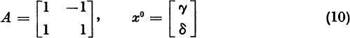
In the complex case (2), the iterates x^k = A^kx⁰ do not approximate eigenvectors as k → ∞.

EXAMPLE 1. Let

 

The eigenvalues are λ₁ = 1 + i, λ₂ = 1 − i. The iterates x⁰, x¹,. . . are

 

The vector x^k+l is found by rotating x^k through 45⁰ and multiplying the length by .

In general, let x⁰ have an eigenvector expansion (3). Even though we are computing complex eigenvalues λ₁ and we will use only real numbers until the last step. We pick for x⁰ a real vector such as the vector defined by (7). The iterate x^k has the eigenvector expansion (4). Let

 

Since for v > 2, the expansion (4) yields

 

where r^k → 0 as k → ∞. Since A and x^k are real, we may assume that and that the eigenvectors u¹ and u² are complex conjugates. We assume that ξ₁ ≠ 0. Note that, for all k, since u¹ and u² are independent,

 

where . Therefore, we have the asymptotic form

 

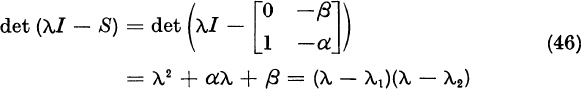
In the complex case for large k, successive vectors x^k do not become multiples of each other. For large k, the vectors x^k lie approximately in the plane spanned by the independent eigenvectors u¹ and u². Therefore, successive triples x^k, x^k+1, x^k+2 are almost dependent. Explicitly, if α and β are the real coefficients of the quadratic

 

then, for all k, , and hence

 

The asymptotic form (14) now yields the approximate equation

 

If we can find the coefficients of dependence α and β we can compute λ₁ and λ₂ as the roots of the quadratic (15):

 

Since λ₁ and λ₂ are complex, α² – 4β < 0.

EXAMPLE 2. In Example 1, Since λ¹ = 1 + i and λ₂ = 1 − i are the only eigenvalues, the iterates (11) satisfy

 

Here α = –2, β = 2, (λ − λ₁)(λ − λ₂) = λ₂ − 2λ + 2.

Computing procedure. In practice, we are given an n × n real matrix A; we assume that we have either the real case (1) or the complex case (2), but we do not know which. If we have the real case, we must compute λ₁; if we have the complex case, we must compute λ₁ and

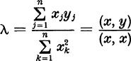
Begin with the vector x = x⁰ defined, say, by (7). Compute the first iterate y = Ax. Now make a least-squares fit of x to y, i.e., choose the real number λ to minimize

 

Setting the derivative with respect to λ equal to zero, we find the value

 

Define a small tolerance > 0, for example, = 10⁻⁵. If the quantities x, y, and λ satisfy

 

we conclude that we have the real case, and we assign the value λ to λ₁.

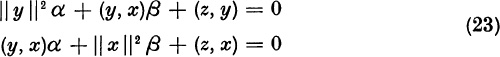
If the test (21) is failed, we compute the third iterate, z = Ay. Pick the real numbers α and β which minimize

 

Calculus gives the necessary conditions

 

The optimal values α and β are found from (23) to be

 

If the quantities x,y, z, α, β satisfy

 

we conclude that we have the complex case, and we assign the root values (18) to λ₁ and λ₂.

Suppose that both the real test (21) and the complex test (25) are failed. Then we must iterate further. If we form the iterates A^kx without some scaling, we may eventually obtain numbers too large or too small for the floating-point representation. The last computed iterate was z = A²x. We scale z by dividing z by the component z_m of largest absolute value. We then define

 

We now repeat the preceding process: We form y = Ax and make the real test (21). If that test is failed, we form z = Ay and make the complex test (25). If the complex test is also failed, we define a new vector x by (26), etc. If is not too small, one of the tests ultimately will be passed. Scaling does not affect the asymptotic equation for x^k = x, x^k+1 = y, and x^k+2 = z:

 

because the equation is homogeneous. The sequence of scaled vectors x; y, z; x, y, z;. . . is simply

 

where σ₁, σ₂,. . . are nonzero scalars.

The method of iteration suffers very little from rounding error. If a new x is slightly in error, we may simply regard this x as a new initial vector which is, no doubt, better than the previous initial vector. Rounding error affects the accuracy of the computed eigenvalues only in the last stage of the computation, when x is fitted to y, or when x and y are fitted to z.

The reader may have wondered why, if we are computing eigenvalues, we do not simply find the coefficients of the characteristic polynomial φ(λ) = det (λI − A). Then the eigenvalues λ_j could be found by some numerical method for solving polynomial equations Indeed, this is sometimes done. But unless an extremely efficient method such as that of Householder and Bauer (see Section 7.12) is used, there is a large rounding error from the extensive computations needed to obtain the n coefficients of from the n² components of A. Even for n = 5 or 6 the rounding error may be quite large.

Moreover, a root λ_j of depends unstably on the coefficients if is small. Infinitesimal variations dc₁. . . , dc_n in the coefficients produce the variation dλ according to the formula of calculus:

 

Since we find

 

PROBLEMS

    1.  Show what happens when the method of iteration is applied to

 

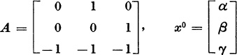
What are the coordinates of the vectors x^k for k = 760, 761, 762, 763 ?

    2.  Suppose that A has a simple eigenvalue λ_i which is known to be approximately equal to −1.83. Form the matrix B = (A + 1.83I)⁻¹, and apply the method of iteration to B. What is the dominant eigenvalue of B ? How can you compute λ_i?

    3.  Suppose that the real matrix A has distinct eigenvalues. Suppose that two of the eigenvalues, λ_i and are known to be approximately equal to 1 ± i. Form the real matrix

 

How can the method of iteration be used to compute λ_j and ?

    4.  Let . Define the rate of convergence to be the reciprocal of the asymptotic value v_e for the number of iterations needed to reduce the error by the factor 1/e. Show that, for the method of iteration,

 

    5.  Let A be a real, symmetric, positive-definite matrix with the eigenvalues λ₁ > λ₂ > ... > λ_n. Suppose that we have computed numerical values for λ₁ and for a corresponding unit eigenvector u¹. If y ≠ a multiple of u¹, form

 

The vector x⁰ is nonzero and is (apart from rounding error) orthogonal to u¹. If there were no rounding error and if u¹ were exact, show that the method of iteration, applied to x⁰, would produce the second eigenvalue, λ₂. Explain why rounding error causes the method of iteration, applied to x⁰, to produce the dominant eigenvalue, λ₁, again.

    6.  In formula (24), the denominator

 

equals zero if and only if the vectors x and y are dependent, as we saw in the proof of the Cauchy-Schwarz inequality. Why are the vectors x and y independent whenever formula (24) is applied in the method of iteration ?

    7.  Let A be a real, symmetric matrix, with eigenvalues .

Let λ be any number satisfying the test for a real eigenvalue:

 

Prove that, for some eigenvalue λ_j,

 

Thus, represents an upper bound for the proportional error. (Expand x in terms of unit orthogonal eigenvectors u¹, . . . , uⁿ.)

   8.* Let A be an n × n matrix with independent unit eigenvectors u¹, . . . , uⁿ. Let T be the matrix with columns u¹, . . .,uⁿ. If

 

prove that, for some eigenvalue λ _j,

 

Use the inequality

 

7.10   REDUCTION TO OBTAIN THE SMALLER EIGENVALUES

In the last section we supposed that A was an n × n real matrix with real and complex eigenvalues λ_l . . . , λ_n. We showed how to compute either a dominant real eigenvalue, λ₁, satisfying

 

or a dominant complex-conjugate pair, , satisfying

 

We will now show how to obtain from A a reduced matrix R whose eigenvalues are the remaining eigenvalues of A. The method of iteration for dominant eigenvalues, when applied to R, yields one or two smaller eigenvalues of A. The matrix R then can be reduced further to a matrix R′, etc., until all the eigenvalues of the original matrix A have been computed.

In the real case (1) the method of iteration yielded quantities λ = λ₁, x, and y = Ax satisfying

 

apart from a negligible error. Suppose for the moment that

 

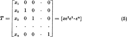
Form the nonsingular n × n matrix

 

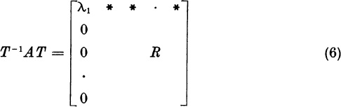
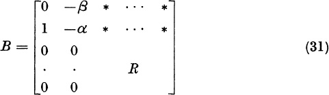
We will show that

 

where the (n − 1) × (n − 1) matrix R has the required property

 

The numbers * in the top row of (6) are irrelevant.

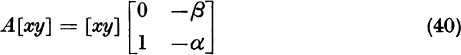
To prove (6), multiply (5) on the left by A. Since Ax = λ₁x and Ae^j = a^j, the jth column of A, we find

 

The matrix B = T^−lAT satisfies the equation TB = AT. If the columns of B are b¹, . . . , bⁿ, then the columns of TB are Tb¹, . . . , Tbⁿ. By (8), the equation TB = AT implies

 

Since x is the first column of T, the solutionof the equation Tb^l = λ₁x is

 

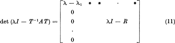
Therefore, B = T ^−lAT has the form (6). The identity (7) follows by taking the characteristic determinants of the matrices on both sides of (6):

 

Recalling the invariance (see Theorem 1, Section 4.2)

 

we find from (11) the identity

 

Division of both sides of (13) by λ − λ₁ yields the required result (7). Note that I in the expression λI − R, is the identity of order n − 1.

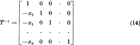
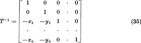
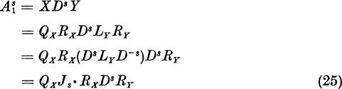
To compute R, we verify that

 

Indeed, since x₁ = 1, the matrix (14) times the matrix (5) equals I. Since R comprises the elements in i, in the product T ⁻¹ AT, we have

 

where X consists of the rows of T ⁻¹, and Y consists of the columns of T. Explicitly,

 

Therefore,

 

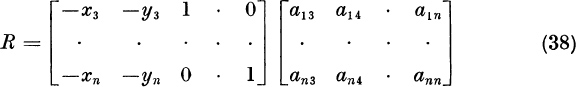
which yields R = (r_ij) in the explicit form

 

Now we shall eliminate the assumption that 1 = x₁ = max | x_i |. This assumption was convenient because it insured that the matrix T, denned by (5), was nonsingular and because it produced no large numbers x_{i + 1} in the final formula (18). Given A, λ₁, and x ≠ 0, we will find a new A and a new x satisfying Ax = λ₁x such that the new A has the same eigenvalues as the old A, and such that the new x does satisfy 1 = x₁ = max | x_i |. Let

 

Since x ≠ 0, we have x_m ≠ 0. The vector u satisfies

 

Let P_ij be the matrix which permutes components i and j of a vector. For example, if n = 3,

 

P_ij is the matrix formed by interchanging rows i and j of the identity matrix. Note that

 

Note also that AP_ij is formed by interchanging columns i and j in A; P_ijA is formed by interchanging rows i and j in A.

Referring to (20), we see that υ = P_lm u is a vector with maximal component υ₁ = 1. Further,

 

But, by (21), PAP = P^−l AP, which has the same eigenvalues as A. Thus, we define

 

The new matrix A and the new vector x have all the required properties, including (4). Note that the new A is formed from A by interchanging rows 1 and m and interchanging columns 1 and m. The reduced matrix R is then computed directly from formula (18).

In the complex case (2), the method of iteration yielded real quantities α, β, x, y = Ax, and z = Ay satisfying

 

We know that x and y are independent because in the testing procedure of the preceding section, the numbers α and β were computed only after the failure of an attempt to express y as a scalar multiple of x ≠ 0. For the moment assume that x and y have the special forms

 

The coefficients α, β satisfy

 

We will find an (n − 2) × (n − 2) matrix R whose eigenvalues are λ₃, . . ., λ_n.

Define the n × n matrix

 

Since Ax = y and Ay = z = − βx − αy,

 

The matrix B = T ^−lAT satisfies TB = AT. If b¹, ... are the columns of B, then by (28)

 

By (27) we conclude that b^l and b² have the forms

 

Therefore, B = T ^−lAT has the form

 

The numbers * are irrelevant. Because of the zeros below the 2 × 2 block in the upper-left corner,

 

Because B is similar to A, B has the same characteristic determinant. Therefore (32) implies

 

The identity λ² + αλ + β = (λ − λ₁)(λ − λ₂) now gives

 

To compute R, we verify that

 

Indeed, since x and y have the special forms (25), the matrix (35) times the matrix (27) equals I. Since R consists of the elements in rows and columns of the product T^−lAT, we have

 

where X consists of the rows of T^−l, and Y consists of the columns of T. Explicitly,

 

Therefore,

 

which yields R = (r_ij) in the explicit form

 

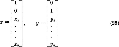
Suppose now that x, y = Ax, and z = Ay satisfy the dependence (24) but that x and y do not have the special form (25). Then x and y are independent vectors satisfying

 

Here [xy] represents the n × 2 matrix with columns x and y. Let N and Q be nonsingular n × n and 2 × 2 matrices. By (40),

 

Set

 

Suppose further that the vectors x′, y′ have the special form

 

In analogy to (27), let T′ be the n × n matrix

 

Equation (41) states that

 

where the 2 × 2 matrix S is denned in (42). Note that

 

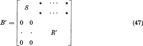
By analogy to (31), B′ = (T′)^−l A′ T′ has the form

 

Therefore,

 

But B′ is similar to A′, which is similar to A. Therefore,

 

Dividing (48) by (λ − λ₁)(λ − λ₂), we find

 

Therefore, R′ is the required reduced matrix. By analogy to (39), we have the explicit form R′ = (r′_ij), with

 

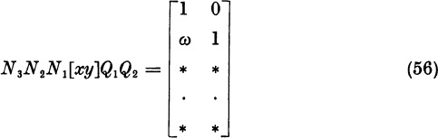
It remains only to find an n × n matrix N and a 2 × 2 matrix Q such that N [xy]Q = [x′y′], where x′, y′ have the form (43). Let

 

Define . Define N₁ = P_1m, the matrix which permutes the first and wth components. Then we have the form

 

Let Q₂ be a 2 × 2 matrix which subtracts η times the first column from the second column:

 

Then, by (53), we have the form

 

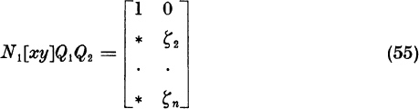
Let ; this maximum is positive because the two columns (55) remain independent. Let N₂ = P_2k, and let N₃ divide row 2 by ζ_k. Then we have the form

 

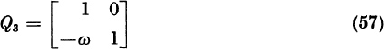
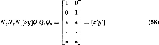
Explicitly, N₃ = diag . Let Q₃ subtract ω times column 2 from column 1:

 

Then we obtain x′, y′

 

There is no need to obtain N = N₃N₂N₁ and Q = Q₁Q₂Q₃ explicitly, but we must obtain A′ = NAN⁻¹ explicitly to compute the reduced matrix R′ from (51). We have

 

since . Formula (59) gives the following procedure. Begin with A. Interchange columns 1 and m. Interchange rows 1 and m. Interchange columns 2 and k. Interchange rows 2 and k. Divide row 2 by ζ_k. Multiply column 2 by ζ_k. The result is A′. Since the vectors x′,y′ were given by (58), we can now compute the reduced matrix from (51).

Although the analysis has been long, the explicit computations (58), (59), (51) are very brief. Therefore, double precision can be used with a negligible increase in computing time. In any case, rounding error is reduced by the choice of the maximal pivot-elements x_m and ζ_k.

PROBLEMS

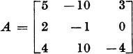
    1.  Let

 

This matrix has the simple eigenvalue λ₁ = 4, with the eigenvector x = col (1, 1, 1). Find the 2 × 2 reduced matrix R.

    2.  Let

 

This matrix has the simple eigenvalue λ_l = −1, with the eigenvector x = col (0, 3, 10). Find the 2 × 2 reduced matrix R.

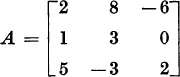
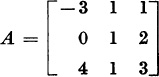
    3.  Let

 

Verify that A²x − 4Ax + 5x = 0. Compute two complex-conjugate eigenvalues. Using formula (51), compute the l × l reduced matrix R. First perform the transformations (58) and (59).

    4.  Let x and Ax be independent; let x, Ax, and A²x be dependent:

 

If λ² + αλ + β ≡ (λ − λ₁)(λ − λ₂), show that (A − λ₂I)x is an eigenvector belonging to λ₁

    5.  Let

 

Verify that x, Ax, and A²x are dependent. Compute two complex eigenvalues, and form the 2 × 2 reduced matrix, R. Then compute the other two eigenvalues of A.

7.11   EIGENVALUES AND EIGENVECTORS OF TRIDIAGONAL AND HESSENBERG MATRICES

Some methods for computing the eigenvalues of an n × n matrix A depend upon finding the coefficients c_j of the characteristic polynomial

 

The eigenvalues are then found by some numerical method for computing the roots of polynomial equations.

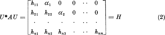
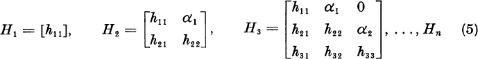
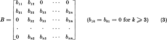
In the method of Householder and Bauer, to be presented in the next section, given A, we construct a unitary matrix U such that the similar matrix U* AU has the special form

 

This is the Hessenberg form, with

 

In particular, if A is Hermitian, then H is Hermitian. A Hermitian Hessenberg matrix H is tridiagonal, with .

The reduction (2) is useful if there is an easy way to find the coefficients of the characteristic polynomial of a Hessenberg matrix, since the identities U*AU = H, U*U = I imply

 

The purpose of this section is to show how to find the coefficients c_j of the characteristic polynomial of a Hessenberg matrix H. As a by-product, we shall show how to find an eigenvector belonging to a known eigenvalue of H. We also will show, in the Hermitian case, that the eigenvalues can be located in intervals without any numerical evaluation of the roots of the characteristic equation.

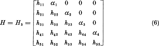
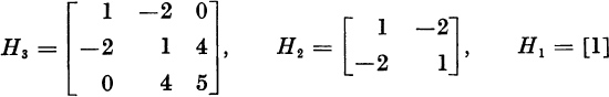
Given H = H_n, construct the sequence of Hessenberg matrices

 

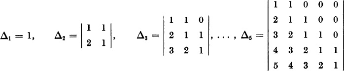
Let Δ₁ = det H₁, . . . , Δ_n = det H_n. We will develop a recursion formula for these determinants.

EXAMPLE 1. For n = 5 we have

 

We shall expand Δ₅ = det H₅ by the last row.

 

Thus, if we define Δ₀ = 1,

 

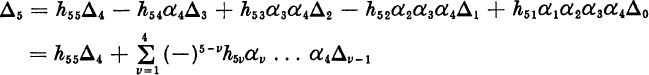
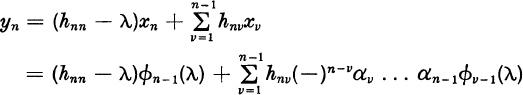
In the general case, expanding Δ_n = det H_n by the last row, we find

 

To find the characteristic polynomial , we only need to replace the diagonal elements h_vv by h_vv − λ. Then (7) yields, for ,

 

where and . This is a formula for computing, successively, , . . . . If H_n is tridiagonal, (8) takes the simpler form

 

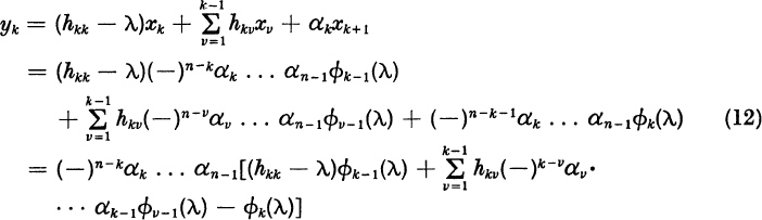
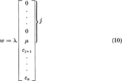
Next we shall show that, if λ is an eigenvalue of H_n, an eigenvector x = col (x₁, . . . , x_n) is given by

 

provided that at least one of these numbers x_i is nonzero. Since x₁ = ±α₁ . . . α_n−1, we have at least x₁ ≠ 0 if all α_v ≠ 0.

To show that (10) provides an eigenvector, we must show that, if , then

 

If y = (H_n − λI)x, then

 

which equals , by (8). For k < n we have

 

But this expression equals 0, as we see by replacing n by k in the recursion formula (8).

If H is Hermitian, with all α_j ≠ 0, we will show how the eigenvalues can be located in intervals. Since , the polynomials , . . . , defined by (9) satisfy

 

Let a < λ < b be a given interval. We suppose that neither a nor b is a zero of any of the polynomials . We will count the number of zeros of in the interval (a, b). Note the following properties:

      (i)    in (a, b). [In fact, .]

     (ii)   If , then and are nonzero and of opposite signs.

Proof. By (13), if either adjacent polynomial, or , is zero, the other one must also be zero. But then and have a common zero, and the recursion formula shows that , etc. Finally, we could conclude , which is impossible. Therefore, implies both and . By (13),

 

Therefore, and have opposite signs.

    (iii)   As λ passes through a zero of , the quotient changes from positive to negative.

Proof: By (ii), the adjacent polynomials and cannot have a common zero. By the inclusion principle (Section 6.4), the zeros μ_j of separate the zeros λ_j of :

 

Furthermore,

 

Therefore, changes sign exactly once, at the pole λ = μ_j, between consecutive zeros λ_j+1, λ_j; and we have Fig. 7.6 as a picture of the algebraic signs of . We see that the sign changes from + to − as λ crosses each λ_j.

Figure 7.6

Sequences of polynomials with properties (i), (ii), (iii) are called Sturm sequences. They have this remarkable property:

Theorem 1. Let be Sturm sequence on the interval (a, b). Let σ(λ) be the number of sign changes in the ordered array of numbers . Then the number of zeros of the function in the interval (a, b) equals σ(b) − σ(a).

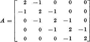
EXAMPLE. Let

 

If and for , then

 

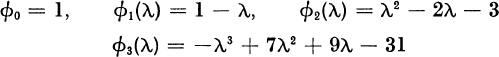
For λ = 0 we have the signs

 

Hence, σ(0) = 1. For λ = 10 we have the signs

 

Hence, σ(10) = 3. The number of zeros of in the interval (0, 10) is, therefore, σ(10) − σ(0) = 3 − 1 = 2.

Proof of Sturm’s Theorem. The function σ(λ) can change only when λ passes through a zero of one of the functions . By property (i), never changes sign in (a, b). If , consider the triple

 

If , property (ii) states that and have opposite signs. Therefore, the triple (14) yields exactly one sign change for all λ in the neighborhood of λ₀. Assume . Then σ(λ) cannot change as λ crosses λ₀.

If λ crosses a zero λ_v of , property (iii) states that the signs of

 

change from + + to + −, or − − to + +. Therefore, exactly one sign change is added in the sequence of ordered values . In other words, σ(λ) increases by 1. In summary, σ(λ) increases by 1 each time λ crosses a zero of ; otherwise, σ(λ) remains constant. Therefore, σ(b) − σ(a) is the total number of zeros of in the interval (a, b).

In practice, Sturm’s theorem can be used with Gershgorin’s theorem (Section 6.8). For tridiagonal H = H*, we know from Gershgorin’s theorem that every eigenvalue of H satisfies one of the inequalities

 

where h₀₁ = h_{n, n+1} = 0. The union of the possibly-overlapping intervals (15) is a set of disjoint intervals

 

These intervals can be subdivided, and Sturm’s theorem can be applied quickly to each of the resulting subintervals (a_iα, b_iα).

When Sturm’s theorem is used numerically to locate the eigenvalues of tridiagonal H = H*, the coefficients of the characteristic polynomials should not be computed. Instead, the recursion formula (13) should be used directly to evaluate successively the numbers and hence the integer σ(λ).

In the proof of Sturm’s theorem, we assumed that

 

We can show that it was only necessary to assume

 

If (18) is true but (17) is false, then for all sufficiently small > 0 we have

 

By what we have already proved, the number of zeros of in (a + , b − ) is σ(b − ) − σ(a + ). But

 

because has no zeros for . Thus, the number of zeros of in (a, b) equals the number of zeros of in (a + , b − ), which equals σ(b) − σ(a).

For a precise computation of the eigenvalues, Newton’s method should be used after the eigenvalues have been separated and approximated by the theorems of Gershgorin and Sturm. Newton’s method for computing the real roots of an equation is discussed in texts on numerical analysis. This method converges extremely rapidly if the first approximation is fairly accurate.

PROBLEMS

    1.  Using the recurrence formula (8), evaluate det (H − λI) for the n × n Hessenberg matrix

    2.  Evaluate successively

 

   3.* Let

 

Define Δ₀ = 1, Δ₁ = c₁,

 

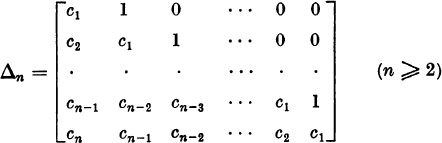
Prove that

 

[Show that (7) implies as in Problem 2, evaluate Δ_n for all n.

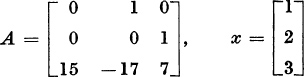
    4.  Using formula (10), calculate an eigenvector for the matrix

 

belonging to the eigenvalue λ = 0.

    5.  Let H be a Hessenberg matrix, as in formula (2). Show that H is similar to a Hessenberg matrix H′ with if if α_j = 0. (Form , where A is a suitable diagonal matrix.)

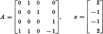
    6.  Let

 

Let . Using the recursion formula (13), calculate numerical values for the for λ = 0 and for λ = 4. How many eigenvalues of A lie between 0 and 4?

   7.* Let H_n be the n × n matrix

 

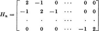
(The matrix A in the last problem is H₅). Let and, for , let . I Making the change of variable λ = 2 − 2 cos θ, prove that

 

Hence find all the eigenvalues of H_n. [Use the recursion formula (13).]

7.12   THE METHOD OF HOUSEHOLDER AND BAUER

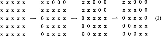
Let A be a real, symmetric n × n matrix. We will show how A can be reduced to tridiagonal form by n − 2 real, unitary similarity-transformations. For n = 5 the process is illustrated as follows:

 

From the tridiagonal form, the characteristic polynomial can be found by the recursion formula (9) of the preceding section, or the eigenvalues can be located in intervals by Sturm’s theorem (Theorem 1, Section 7.11).

If A is real but not symmetric, the method will produce zeros in the upper right corner but not in the lower left corner. For n = 5, the process would appear as follows:

 

The final matrix is in the Hessenberg form, and the characteristic polynomial can be found by the recursion formula (8) of the last section. If A is complex, the method is modified in the obvious way, by replacing transposes x^T by their complex conjugates x*.

In the real, symmetric case, the first transformation A → B = U^TA U is required to produce a matrix of the form

 

If all a_1k already , we set B = A. Otherwise, we will use a matrix of the form

 

Explicitly, if the real column-vector u has components u_i, then U = (δ_ij − 2u_iu_j). Since we require u to have unit length, U is unitary.

 

U is also real and symmetric: U^T = U. The requirements

 

place n − 1 constraints on the n-component vector u. Since there is one degree of freedom, we set u₁ = 0. Note that b_lk = 0 implies b_kl = 0, since B is symmetric.

The first row of B = UAU is the first row of UA times U. Since u₁ = 0, the first row of U = I − 2uu^T is just (1,0, . . ., 0). Therefore, the first row of UA is just the first row of A. Hence, the first row of B is

 

Since U = I − 2uu^T, we have a^TU = a^T − 2(a^Tu)u^T, or

 

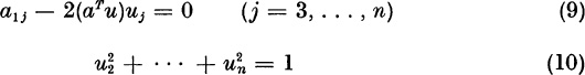
The unknowns u₂, . . . , u_n must solve the n − 1 equations

 

To solve these equations, we observe that the rows a^T and b^T = a^TU must have equal lengths: b^Tb = a^TUU^Ta = a^Ta. Thus, we require

 

By (8), b₁₁ = a₁₁. Then (11) takes the form

 

If , equations (8) and (12) yield

 

We now multiply (13) by u₂, (9) by u_j (j = 3, . . . , n), and add to obtain

 

or

 

or, since we require u^Tu = 1,

 

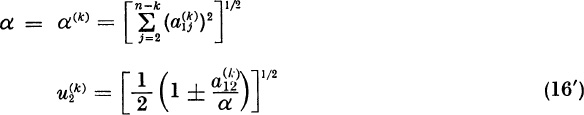
This is a relationship between the unknown inner product a^Tu and the unknown component u₂. Using (14) in the identity (13) for b_l2, we find

 

We have α > 0 because at least one . Therefore, (15) has the positive solution

 

We choose the sign ± so that . Since α > | a₁₂ |, we have . Having computed u₂, we compute u₃. . . , u_n from (9) and (14).

 

Exercise If ± is chosen so that , and if we define

 

verify directly that the numbers u₂, . . . , u_n defined by (16) and (17), solve the required equations (9) and (10).

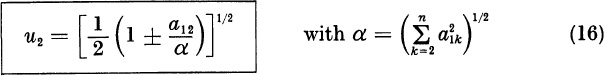
We now transform A into B = UAU, with b_lk = b_kl = 0 for . If n > 3, we wish next to transform B into a matrix C = VBV with

 

We shall require V^TV = I and V = V^T.

Observe the matrix B in (3). We can partition B as follows:

 

where A′ is the (n − 1) × (n − 1) matrix . By analogy to (16) and (17), we can reduce A′ to the form

 

by a transformation B′ = U′A′U′, where

 

If A′ has not already the form (21), we simply define

 

and define, in analogy to (16) and (17),

 

The sign ± is chosen to make .

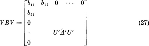
We now assert that the required matrix V has the form

 

Proof: Since , the matrix V has the form

 

The first row of VBV is the first row of V times BV. Since the first row of V is (1, 0, . . . , 0), the first row of VBV is just the first row of B times V, or

 

Here we have used the form (25) for V. Thus, the first row and, by symmetry, the first column are unaffected. The partitoned form (24) now shows that

 

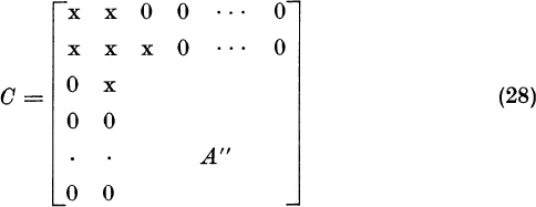
But U′A′U′ = B′ of the form (21). Therefore, VBV = C of the required form

 

where A″ is an (n − 2) × (n − 2) symmetric matrix.

We note parenthetically that V in (24) has the form

 

where υ is the unit vector col .

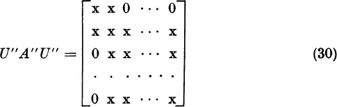
The process now continues. Let U″ be the (n − 2) × (n − 2) matrix of the form I″ − 2u″(u″)^T which reduces A″ to the form

 

We then define

 

Since , this matrix has the form

 

Therefore, as (28) shows, the first two rows and the first two columns are unaffected by the transformation C → WCW. Therefore,

 

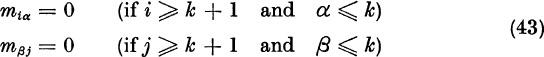
After k reductions we obtain a symmetric n × n matrix, say Z = (z_ij), with

 

We call A^(k) the lower-right part.

 

If k < n − 2, we will reduce Z further. If at least one of the numbers is nonzero, we form from (16) and (17), replacing A by A^(k), and n by n − k. Setting we have the form

 

where

 

If we define the n × n matrix

 

we must show that the first k rows and the first k columns of Z are unaffected by the transformation Z → MZM = Z′. Now

 

Let Then by (38), and

 

By (34), . Therefore, (39) yields

 

But (38) shows that

 

Then (40) implies if . By symmetry, we also have if .

Finally, we must show that Z′ = MZM implies

 

Now the form (38) shows that

 

Therefore,

 

But (44) is equivalent to (42), since

 

COMPUTING ALGORITHM

The preceding three paragraphs give a rigorous justification of the method. In practice, the matrix M in (38) is not formed explicitly, nor is the matrix U^(k)

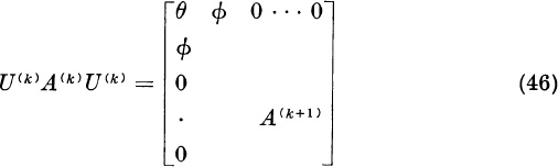
At each stage k = 0, 1, . . . , n − 3 our task is to replace the (n − k) × (n − k) matrix A^(k) by the matrix

 

The number θ is unchanged = . If, by chance,

 

then no computation is performed at stage k, since A^(k) already has the form of the right-hand side of (46). Otherwise, we do compute the numbers by (16) and (17), replacing A by A^(k), and n by n − k. Dropping the superscript k, we observe that

 

Define the quadratic form

 

Compute Au = b, i.e., compute

 

By (48), the i, j-component of U^(k) A^(k) U^(k) is

 

Replace by

 

Replace by 0, . . . , 0. For replace by the following equivalent of (51):

 

where

 

The components with i > j are now formed by symmetry,

COUNT OF OPERATIONS

We will count the number of multiplications and the number of square roots. At stage k = 0,1, . . . , n − 3, the calculations

 

 

require 2 square roots and approximately 2(n − k) multiplications. To form b in (50) requires (n − k)(n − k − 1) multiplications. The calculation of c requires n − k − 1 multiplications. The calculations (53) require

 

which is equal to (n − k) (n − k − 1) multiplications. In summary, at stage k there are

 

Summing for k = 0, . . . , n − 3, we find a total of

 

Thus, there are very few multiplications. After all, just to square an n × n matrix requires n³ multiplications. Since the number of multiplications is small, it will usually be economically feasible to use double precision.

PROBLEMS

    1.  Reduce the matrix

 

to tridiagonal form by the method of Householder and Bauer.

    2.  Reduce the matrix

 

to Hessenberg form by the method of Householder and Bauer.

   3.* Reduce the matrix

 

to tridiagonal form by the method of Householder and Bauer.

   4.* According to formula (55), the H-B reduction of an n × n symmetric matrix requires “about” 2n³/3 multiplications. What is the exact number of multiplications?

    5.  If A is real but not symmetric, and if A is to be reduced to Hessenberg form by the H-B method, how should formulas (50)–(53) be modified?

    6.  If a real matrix A is reduced to a tridiagonal or Hessenberg matrix X by the H-B method, show that . (This identity can be used as a check of rounding error.)

7.13   NUMERICAL IDENTIFICATION OF STABLE MATRICES

In the theory of automatic control, in circuit theory, and in many other contexts the following problem arises: Given an n × n matrix A, determine whether all of its eigenvalues lie in the left half-plane Re λ < 0. The matrix A is called stable if all of its eigenvalues lie in the left half-plane. The importance of this concept is shown by the following theorem:

Theorem 1. An n × n matrix A is stable if and only if all solutions x(t) of the differential equation

 

tend to zero as t → ∞.

Proof. Suppose that A has an eigenvalue λ with Re . If c is an associated eigenvector, then the solution

 

does not tend to zero as t → ∞ because .

Suppose, instead, that A is stable. Let λ₁ . . . , λ_s be the different eigenvalues of A, with multiplicities m₁ . . . , m_s. In formula (17) of Section 5.1, we showed that every component x_v(t) of every solution x(t) of the differential equation dx/dt = Ax is a linear combination of polynomials in t times exponential functions exp, λ_it. Since all λ_i have negative real parts, every such expression tends to zero as t → ∞. This completes the proof.

One way to show that a matrix is stable is to compute all its eigenvalues and to observe that they have negative real parts. But the actual computation of the eigenvalues is not necessary. By results of Routh and Hurwitz, it is only necessary to compute the coefficients c_i of the characteristic polynomial

 

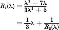
Assume that A is real, andhence that the c_i are real. Form the fraction

 

If c₁ ≠ 0, this fraction can be rewritten in the form

 

where α₁ = 1/c₁ and

 

with

 

Similarly, we write

 

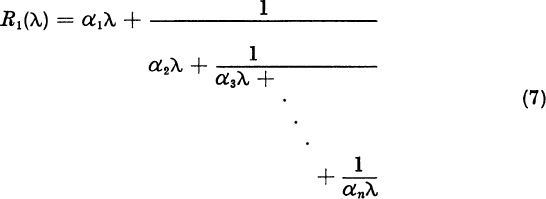
and so on until we obtain the full continued fraction

 

Theorem 2. The zeros of the polynomial λⁿ + c₁λⁿ⁻¹ + ... + c₀ all lie in the left half-plane if and only if the coefficients α₁ in the continued fraction (7) are all positive.

EXAMPLE 1. Consider the polynomial

 

We have

 

with

 

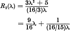
The full continued fraction is

 

Here

 

Since all α_i are positive, Routh’s theorem states that the zeros λ_v of the polynomial (8) are in the left half-plane. In fact, the zeros are

 

We will not prove Routh’s theorem, which is not a theorem about matrices, but a theorem about polynomials. A proof and a thorough discussion appear in E. A. Guillemin’s book, The Mathematics of Circuit Analysis (John Wiley and Sons, Inc., 1949) pp. 395–407. If the n × n matrix A is real, and if n is small, Routh’s theorem provides a practical criterion for the stability of the matrix A. But if n is large, Routh’s theorem is less useful because it is hard to compute accurately the coefficients of the characteristic polynomial. If the coefficients c_i are very inaccurate, there is no use in applying Routh’s theorem to the wrong polynomial.

A second criterion, which applies directly to the matrix A, and which does not require that A be real, is due to Lyapunov.

Theorem 3. The n × n matrix A is stable if and only if there is a positive definite Hermitian matrix P solving the equation

 

If n is large, this theorem is hard to use numerically. The system (9) presents a large number, n(n+ l)/2, of linear equations for the unknown components . One must then verify that P is positive definite by the determinant criterion (see Section 6.5)

 

Because Lyapunov’s theorem has great theoretical interest, we shall give the proof.

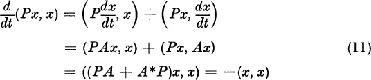
Proof. First assuming PA + A*P = –I, we shall prove that A is stable. By Theorem 1, it will be sufficient to show that every solution of the differential equation dx/dt = Ax tends to zero as t → ∞. We have, for the solution x (t),

 

Since P is positive definite, there is a number ρ > 0 for which

 

Then (11) yields

 

Therefore,

 

If x(0) = b, we conclude that , and hence

 

But for some σ >0. Therefore,

 

which shows that x → 0 as t → ∞.

Conversely, supposing that A is stable, we shall construct the positive-definite matrix P solving PA + A*P = –I. Let the n × n matrix X (t) solve

 

As in the proof of Theorem 1, we know that every component of the matrix X (t) is a linear combination of polynomials in t (possibly constants) times exponential functions exp where Re We bear in mind that the adjoint matrix A* has the eigenvalues if A has the eigenvalues λ_v. Taking adjoints in (17), we find

 

Now the product X (t)X*(t) satisfies

 

Define the integral

 

This integral converges because every component of the integrand has the form

 

which is a linear combination of polynomials in t times decaying exponential functions. By integrating equation (19) from t = 0 to t = ∞, we find

 

The left-hand side, – I, appears because XX* equals I when t = 0 and equals zero when t = ∞. The matrix P is positive definite because the quadratic form belonging to a vector z ≠ 0 equals

 

This completes the proof.

Lyapunov’s theorem shows that, if a matrix A is stable, then there is a family of ellipsoidal surfaces (Pz, z) = const relative to which every solution of dx/dt = Ax is constantly moving inward. In fact, (11) shows that

 

A PRACTICAL NUMERICAL CRITERION

Let us suppose that A is an n × n matrix, not necessarily real, with n large. We will give a criterion for the stability of A which

      (a)  does not require explicit computation of the eigenvalues;

      (b)  does not require explicit computation of the coefficients of the characteristic polynomial; and

      (c)  does not require the solution of systems of N linear equations with

If A has eigenvalues λ₁, . . . , λ_n, and if τ is any positive number, the numbers

 

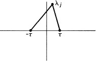
all lie in the unit circle | μ | < 1 if and only if all the numbers λ_j lie in the left half-plane. This is evident from Figure 7.7.

Figure 7.7

The absolute value | μ_j | equals the distance of λ_j from – τ divided by the distance of λ_j from τ. In the figure Re λ_j > 0; therefore | μ_j | > 1.

The numbers μ_j are the eigenvalues of the n × n matrix

 

unless τ = some λ_j. Proof:

 

Assume that τ > 0 has been chosen. The problem now is to determine whether all the eigenvalues μ_j of the matrix B lie inside the unit circle | μ_j | < 1. By Theorem 3 in Section 4.9, all | μ_j | < 1 if and only if

 

In principle, we could form the powers B^k, but we prefer not to do so because each multiplication of two n × n matrices requires n³ scalar multiplications.

We prefer to form the iterates B^kx⁽⁰⁾ = x^(k), where x⁽⁰⁾ is some initial vector. As the vectors x⁽⁰⁾, x^(l), x⁽²⁾, . . . are computed, we look at the successive lengths squared:

 

If these numbers appear to be tending to zero, we infer that A is stable; if these numbers appear to be tending to infinity, we infer that A is unstable; if the numbers || x^(k) ||² appear to be tending neither to 0 nor to ∞, we infer that A is stable or unstable by a very small margin. We will justify this procedure in Theorem 4.

If A is a stable normal matrix—e.g., a stable Hermitian matrix—the numbers (28) will form a monotone decreasing sequence. We see this from the expansion

 

of x⁽⁰⁾ in the unit orthogonal eigenvectors u^j of A. The vectors u^j are also eigenvectors of B. Then

 

where all | μ_j | < 1. If A is not a normal matrix, the sequence (28) will not usually be monotone.

How large should the number τ > 0 be chosen? If τ is too small or too large, all of the eigenvalues

 

of B are near ±1. If any λ_j has Re λ_j > 0, we would like the modulus | μ_j | to be as large as possible. We assert that, if Re λ > 0, then

 

Proof. If λ = ρe^iθ, with | θ |< π/2, we must show that

 

This is true if

 

or if

 

which is true, with equality only if τ = ρ. If A is given, a reasonable first guess for the modulus, ρ, of an eigenvalue is

 

We find this value by summing

 

for i = 1, . . . , n, and by falsely replacing all a_ij by | a_ij | and all x_i by 1. The number τ defined by (30) is of the right general size.

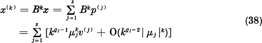
Lemma. Let B be an n × n matrix. Let p be a principal vector of grade belonging to the eigenvalue μ. Then for large k we have the asymptotic forms

 

where v is an eigenvector belonging to μ and where the remainder r^(k) equals 0 if g = 1 or equals

 

Proof. By the notation (32) we mean that, for some constant γ > 0,

 

If g = 1, then p is an eigenvector, p = υ, and r^(k) = 0 in (31). If , we have for

 

In the expansion by the binomial theorem, we have

 

for the principal vector p. The vector

 

is an eigenvector because p has grade g. Since g is fixed as k → ∞, we have

 

For the other terms in (33) we have in the formula

 

The last three formulas yield the required asymptotic form (31).

In the following theorem, we shall use the phrase “with probability one,” and we wish now to define the sense in which this phrase will be used. Consider an arbitrary nonzero n-component vector x. Let B be an n × n matrix with the different eigenvalues μ₁ . . . , μ_s with multiplicities m₁ . . . , m_s, where Σ m_i = n. As we showed in Section 5.2, the vector x has a unique expansion

 

in principal vectors p^(j) belonging to the eigenvalues μ_j. In the last paragraph of Section 5.3 we concluded that the space of principal vectors p^(j) has dimension m_j. Let Z_j be the linear space of vectors x for which p^(j) = 0 in the representation (36). Then the dimension of Z_j is n − m_j < n. Thus, Z_j has n-dimensional measure zero. The set Z of vectors x for which at least one p^(j) = 0 in the expansion (36), is the union

 

of the sets Z_j, all of which have measure zero. Therefore, Z has measure zero. In this sense we say that, with probability one, all of the principal vectors p^(j) are nonzero in the expansion (36) of a random vector x.

Theorem 4. Let B be an n × n matrix. Let x = x⁽⁰⁾ be a random vector.

Let

 

x⁽¹⁾ = Bx⁽⁰⁾, x⁽²⁾ = Bx⁽¹⁾, x⁽³⁾ = Bx⁽²⁾, . . .

Let μ₁, μ₂, . . . be the eigenvalues of B

          Case 1.  if all | μ_j | < 1, then x^(k) → 0 as k → ∞.

          Case 2.  If all , and if at least one | μ_j | = 1, then with probability one the sequence x^(k) does not tend to zero.

          Case 3.  If at least one | μ_j | > 1, then with probability one || x^(k) || → ∞ as k → ∞.

Proof. In Case 1 we know that B^k → 0 as k → ∞, and therefore

 

Let μ₁, . . . , μ_s be the different eigenvalues of B, with multiplicities m₁ . . . , m_s. Let

 

where Σ m_i = n and . Form the expansion (36) of x as a sum Σ p^(j) of principal vectors of B. With probability one all p^(j) ≠ 0. In other words, with probability one every p^(j) in the expansion x = Σ p^(j) has grade . Then, by the preceding lemma,

 

where υ⁽¹⁾, . . . , υ^(s) are eigenvectors corresponding to μ₁ . . . , μ_s. Let

 

Let J be the set of integers j such that and such that g_j = g. Then (38) yields

 

where ρ = | μ_l | = . . . = | μ_r |. By the notation o(K^g−1 ρ^k) we mean any function of k such that

 

For all j ∈ J we have | μ_j | = ρ. Let

 

where the angles θ_j are distinct numbers in the interval . In Cases 2 and 3 we assume . From (40) we have

 

Eigenvectors υ^(j) belonging to different eigenvalues μ_j are linearly independent. Therefore, the minimum length

 

is a positive number δ > 0. Letting α_j = exp (ikθ_j) in (43), we find

 

In Case 2 we have ρ = 1, and || x^(k) || → ∞ if g > 1. If g = 1 and ρ = 1, then (43) shows that x^(k) remains bounded but (45) shows that x^(k) does not tend to zero. In Case 3 we have ρ > 1, and (45) shows that || x^(k) || → ∞.

PROBLEMS

    1.  Let A be an n × n matrix. Let and ψ(λ) be polynomials with real or complex coefficients. Suppose that ψ(λ_j) ≠ 0 for all eigenvalues λ_j of A. Prove that the n × n matrix ψ(A) has an inverse. Then prove that the eigenvalues of the matrix are . (First prove the result for triangular matrices T. Then use the canonical triangularization A = UTU*.)

    2.  Find the Lyapunov ellipses (Px, x) = const for the stable matrix

 

    3.  Let A be any stable n × n matrix and let Q be any n × n positive-definite Hermitian matrix. Show that there is a positive-definite matrix P solving the equation − Q = A*P + PA.

    4.  Let A be any stable n × n matrix. Let C be an arbitrary n × n matrix. Show that the equation −C = A*M + MA has a solution M. Since every equation −C = A*M + MA has a solution, M, deduce that the particular equation −I = A*P + PA has a unique solution, P.

    5.  Let λ³ + c₁λ² + c₂λ + c₃ have real coefficients. According to the Routh-Hurwitz criterion, what inequalities are necessary and sufficient for the zeros of the polynomial to have negative real parts?

    6.  For the stable matrix A in Problem 2, compute the number T in formula (30). Compute the matrix B in formula (26). What are the eigenvalues of B?

    7.  Let

 

Compute the number τ and the matrix B. For which vectors x do the iterates B^kx tend, in length, to infinity as k → ∞? What is the probability, for a random vector x, that || B^kx || → ∞ as k → ∞?

7.14   ACCURATE UNITARY REDUCTION TO TRIANGULAR FORM

In the QR method of computing eigenvalues, we shall need an accurate way of reducing an n × n matrix A to a right-triangular matrix R by transformation

 

Here we assume that A, U, and R are real or complex matrices, with

 

In principle, we could perform this transformation by the Gram-Schmidt process described in Section 4.5. If the columns a¹, . . . , aⁿ of A were independent, we could form unit vectors υ¹, . . ., υⁿ such that a^k would be a linear combination of υ¹, . . . , υ^k.

 

In other words.

 

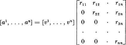
or

 

A = VR

Then we could take U = V* in (1). Unfortunately, the Gram-Schmidt process has been found to be highly inaccurate in digital computation. This inaccuracy is demonstrated in J. H. Wilkinson’s book.²

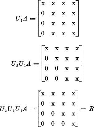
In this section, we shall show how to perform the reduction UA = R by a sequence of reflections

 

where each U_j has the form I − 2ww*, or where U_j = I. Here w is a unit vector depending on j. The matrices U_j are both unitary and Hermitian:

 

The matrix U_j will produce zeros below the diagonal in column j; and U_j will not disturb the zeros which shall already have been produced in columns 1, . . . , j – 1. Thus, if n = 4,

Let A₁ = A, and for j > 1 let

 

A_j = U_{j − 1}. . . U₁A

Assume that A_j has zeros below the diagonal in columns 1, . . . , j − 1. Let the j th column of A_k have the form

 

Let

 

If β = 0, then A_j already has zeros below the diagonal in column j, and we set U_j = I.

If β > 0, we look for U_j in the form

 

We shall have

 

For this vector to have zeros in components j + 1, . . . , n, we must have w_j+1, . . . , w_n proportional to c_j+1, . . . , c_n, since 2(w*c) is simply a scalar.

Thus, we look for w in the form

 

Then

 

and U_jC will have zeros in components j + 1, . . . , n if

 

For w to be a unit vector, we must have

 

Elimination of | λ |² from (11) and (12) gives

 

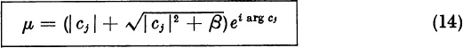
If c_j = | c_j | exp (iγ_j), we will look for μ in the form μ = | μ | exp (iγ_j). Then (13) becomes

 

which has the positive solution

 

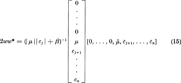
Then

 

Now (11) yields

 

and hence

 

Then U_j = I – 2ww*.

We must show, finally, that multiplication by U_j does not disturb the zeros below the diagonal in columns 1, . . . , j − 1. If z is any of the first j − 1 columns of A_j, then z_j = z_j+l = . . . = z_n = 0. Therefore,

 

Now (15) shows that the first j − 1 columns of A_j are not changed in the multiplication U_jA_j.

We also observe that, since 2ww* has zeros in rows 1, . . . , j − 1, the first j − 1 rows of A_j are, likewise, not changed in the multiplication U_jA_j.

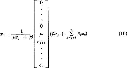
To perform the multiplication U_jA_j, we do not first form the matrix U_j. If x is the kth column of , then the kth column of the product U_jA_j is

 

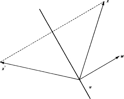
In real Euclidian space, the matrix I − 2ww* represents the easily-visualized geometric transformation in Figure 7.8. Through the origin there is a plane, π, to which w is a unit normal. The vector (w*x)w is the projection of x in the direction of w. If we subtract twice this projection from x, we obtain the vector

Figure 7.8

 

which is the reflection of x through the plane π.

PROBLEMS

    1.  Let α, β, γ, δ be real. Let

 

Reduce A to right-triangular form by a transformation (I − 2ww*)A = R.

    2.  Using the method described in this section, reduce the matrix

 

to right-triangular form.

7.15   THE QR METHOD FOR COMPUTING EIGENVALUES

In this section we will present an introduction to the method of Francis and Kublanovskaya, known as the QR method. We wish to compute the eigenvalues of an n × n real or complex matrix A. By the method of the preceding section, we factor A in the form

 

where Q₁ Q₁* = I and where R₁ is right-triangular. Setting A = A_l, we now form

 

We now factor A₂ in the form A₂ = Q₂ R₂, and we form A₃ = R₂ Q₂. In general,

 

Under certain conditions on A, as s → ∞ the matrix A_s becomes a right-triangular matrix with the eigenvalues of A on the diagonal. We will prove this convergence in the simplest case; we shall assume that A has eigenvalues with distinct moduli:

 

This proof and more general proofs have been given by Wilkinson.3

First, we discuss the transition from A_s to A_s+l. By the method of the preceding section, we can find unitary, Hermitian matrices U₁, . . ., U_{n − 1}, depending on s, such that

 

Thus, A_s = Q_s R_s, where Q_s = U₁ . . . U_{n − 1}. Then

 

The matrix Q_s is never computed explicitly, nor are the matrices U_j. We know that each U_j has the form

 

as in formula (15) of the preceding section. We do compute the scalars and vectors ζ_j and q^(j), and by means of them we compute successively

 

Then we compute successively

 

Every product X(I – ζqq*) occurring in (8) is computed as X – ζyq*, where y = Xq.

We shall now study the uniqueness and the continuity of QR factorizations.

Lemma 1. Let Abe a nonsingular matrix with two QR factorizations

 

where the Q’s are unitary and the R’s are right-triangular. Then there is a diagonal matrix of the form

 

such that

 

Proof. First suppose that Q = R, where

 

Then I = Q*Q = R*R. The first row of R*R is

 

r₁₁(r₁₁,r₁₂, . . . , r_1n)

Therefore,

 

Since r₁₂ = 0, the second row of R*R is

 

Therefore,

 

Continuing in this way, we verify that r_ij = δ_ij(i, j = 1, . . . , n). Therefore, Q = R = I.

If A = Q₁ R₁ = Q₂ R₂, where A is nonsingular, then R₁⁻¹ exists and

 

If the diagonal elements of the right-triangular matrix R₂ R₁⁻¹ have arguments θ_l, . . . , θ_n, and if E is defined by (10), then the matrices

 

satisfy the conditions (12), and Q = R. Therefore, Q = R = I, and the identities Q₂ = Q₁E*, R₂ = ER₁ follow.

Lemma 2. Let A_k → I as k → ∞. Let A_k = Q_kR_k, where Q_k is unitary, and where R_k is right-triangular with positive-diagonal elements. Then Q_k → I and R_k → I as k → ∞.

Proof. We have

 

Let r_ij(k) be the i, j component of R_k. The first row of is

 

Hence,

 

The second row of is

 

Using the first result (15), we conclude that

 

Continuing by successive rows in this way, we conclude that R_k → I as k → ∞. The explicit form of the inverse . (cofactor matrix)^T now shows that , and hence also as k → ∞.

Lemma 3. If Q₁, Q₂, . . . are unitary, and if R₁, R₂, . . . are right-triangular, and if

 

then, for s = 2, 3, . . . ,

 

and

 

Proof. The identities (17) imply that

 

Therefore, if (18) is true for any s, we have

 

Since (18) is true for s = 1, it is true for all s.

Formula (19) also follows by induction from (17), since

 

Theorem 1. Let A₁ be an n × n matrix with eigenvalues λ_j such that |λ ₁| > |λ ₂| > · · · > |λ _n| > 0. Let A₁ have a canonical diagonalization

 

where D = diag (λ₁, . . . , λ_n). Assume that all of the n principal minors of the matrix Y = X⁻¹ are nonsingular:

 

Let matrices A₂, A₃, . . . be formed by the QR method (17). Then there is a sequence of diagonal matrices E₁, E₂, . . . of the form (10) such that

 

where the matrix R_x is right-triangular.

In this sense, A_s tends to a right-triangular matrix with the eigenvalues of A, in order, appearing on the main diagonal.

Proof. As we proved in Section 7.3, the condition (21) is necessary and sufficient for the matrix Y = X⁻¹ to have a decomposition Y = L_Y R_Y, where L_Y is left-triangular, where R_Y is right-triangular, and where L_Y has 1’s on the main diagonal. Then

 

But

 

since the elements above the diagonal are zero, while the elements on the diagonal are 1’s, and the elements below the diagonal satisfy

 

Let X have the factorization X = Q_x R_x where Q_x is unitary and R_x is right-triangular. Then

 

where

 

Since J_s → I as s → ∞, J_s has a QR factorization

 

where is unitary and is right-triangular; that follows from Lemma 2. Then has the QR decomposition

 

But Lemma 3 gives the QR decomposition

 

Now Lemma 1 states that there is a matrix E_s of the form (10) such that

 

Now the identity (19) for A_s yields

 

But

 

Therefore,

 

and

 

This is the justification of the QR method in the simplest case. It is possible to remove the restriction that X⁻¹ have nonsingular principal minors. It is even possible to remove the restriction that the eigenvalues of A have distinct moduli. If the moduli are not distinct, the matrices A_s tend to block-right-triangular matrices, where each m × m block centered on the diagonal is an m × m matrix whose m eigenvalues are eigenvalues of equal moduli belonging to A. The theory underlying this method is surprisingly difficult.

The idea for the QR method came, no doubt, from an older method due to Rutishauser:

 

where L₁, L₂, . . . are left-triangular and R₁, R₂, . . . are right-triangular.

PROBLEMS

In the following problems, assume that all matrices L are left-triangular matrices with 1’s on the main diagonal, and that all matrices R are right-triangular matrices.

    1.  If A = L₁R₁ = L₂R₂, and if A is nonsingular, prove that L₁ = L₂ and R₁ = R₂.

    2.  If A_k = L_kR_k → I as k → ∞, prove that L_k → I and R_k → I.

    3.  If A₁ is a nonsingular matrix, and if

 

prove that

 

   4.* Let A₁ satisfy the conditions of Theorem 1. Assume that matrices A₂, A₃, . . . can be formed as in the last problem. Show that, as s → ∞, A_s tends to a right-triangular matrix whose diagonal elements are the eigenvalues A₁.

---

² J. H. Wilkinson, Rounding Errors in Algebraic Processes. Englewood Cliffs, N.J.: Prentice-Hall, Inc., 1963, pp. 86–91.

³ J. H. Wilkinson, “Convergence of the LR, QR, and related algorithms,” The Computer Journal, vol. 8 (1965), 77–84.