• • • •
So far, we have discussed only a very small part of our genome. The mtDNA genome is only sixteen thousand base pairs in length, with a miniscule thirteen protein-coding genes; and while the Y chromosome is much larger, clocking in at fifty million base pairs, it still only has a paltry seventy or so genes. The Y chromosome is known as a “sex chromosome,” because biological sex in humans (and most mammals) is determined by its presence or absence. Your mother has two X chromosomes, and will always pass an X along to you. Your father has one X and one Y chromosome, so the X you get from your mother will be paired with either an X or a Y from your father; and if you happen to get a Y, your biological sex (that is, what genitalia you develop) will be male. Sexual identity is another issue altogether; but whether you have male or female genitalia is controlled by the presence or absence of the Y chromosome.
The approximately fifty million base pairs in a Y chromosome represent a rather unimpressive 1.6 percent of all the three billion bases in a human genome. The X chromosome, the other “sex-limited genetic element,” is rather bigger; but the vast bulk of our genome resides in the other 22 pairs of chromosomes, known as “autosomes.” That other 98.4 percent of your DNA harbors an immense amount of variation. What is more, while the two DNA markers we have just discussed are clonal, so that the only variation that is introduced to the next generation is caused by mutation, this other DNA experiences what is known as “recombination,” a process that jumbles the alleles that a mother and father pass on to their off-spring. This occurs because the maternal and paternal DNA exchange information, and thereby create new genomic variation without mutation. Via this process the autosomal chromosomes become mosaics of the chromosomes inherited from their ancestors, something that poses a major problem when one tries to analyze the history of organisms—although it certainly doesn’t mean that figuring out the histories of the chromosomes and their mosaic parts is impossible. What it does mean is that each little chunk of DNA on your chromosomes has a unique history. It is as if thousands and thousands of different histories are floating around in a single genome.
Sequencing the first human genomes was a very labor-intensive and expensive process. The best estimate for the cost of sequencing the first couple of human genomes is in the billions of dollars. This high cost was due to the technology used, a brilliant but cumbersome process called Sanger sequencing (named after Fred Sanger, the double Nobel laureate who invented the technology). It required the target DNA to be broken into millions and millions of small fragments, each between five hundred and one thousand bases long—with one thousand being the longest fragment the technique could deal with. With three billion bases in the genome to sequence, a few at a time, this was obviously very time-consuming. But techniques were developed early in this century to parallelize the sequencing steps and allow hundreds of thousands of small fragments to be sequenced simultaneously. This approach allowed the genome of James Watson (codiscoverer of the structure of DNA) to be sequenced at a cost of a million dollars. Subsequent improvements of the technology now permit billions of small fragments of DNA to be sequenced at a time. In addition, techniques have been developed in which breaking the target DNA into small fragments is not necessary. These are known collectively as “next-generation sequencing” (NGS), and they have brought down the cost of sequencing a full human genome to about $1,000.
Since most of the bases in our three billion-base genomes are identical from one human to the next, “targeted sequencing” was an obvious way to expedite assays of individual human genomes for variation. This approach focuses exclusively on those positions in the genome that are variable and thus informative for human genome projects. It is based on the identification of positions in the genome that are polymorphic over a wide range of humans. Figure 8.1 shows a hypothetical set of sequences of the same small stretch of the human genome. Three positions in the sequence are polymorphic, and only one would be targeted as a single-nucleotide polymorphism (SNP). This position would be a good one for targeted sequencing or placement on a sequencing array.
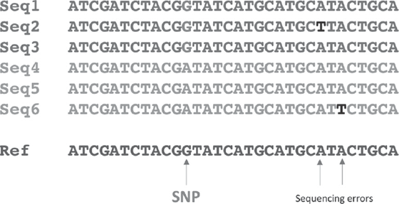
Figure 8.1 Hypothetical sequences from six individuals in two populations. The eighth position (in red) on the left is fixed and differs in the two populations and would be considered an SNP ripe for further analysis. The last two positions from the right (in black) differ in only one individual each and more than likely are caused by sequencing errors or other anomalies. See plate 5.
For targeted sequencing, probes homologous to the sequence of interest are synthesized and hybridized to DNA isolated from the individual being studied. A molecule called biotin is attached to each. There are thousands of such probes, homologous to all the regions of the genome that have SNPs and thus are of interest to researchers. Small magnetic beads bearing molecules that will bind biotin are then mixed with the DNA, and any piece of double-stranded DNA that has biotin on it will bind to one of them. A magnet is then used to separate all the beaded molecules from the rest of the mixture, and all the pieces of DNA that do not contain SNPs of interest are washed away. The beads are then removed, and the DNA is sequenced using the NGS techniques. An alternative “array” approach uses a different technology but also detects targeted SNPs. The targeted sequencing approach is perhaps the more accurate, because it allows for replication sequencing at about 100× coverage (where “coverage” refers to the number of data points for a single SNP).
Typically, several hundred thousand SNPs can be assayed by these methods. The panels are commercially available, and some are proprietary. For instance, Affymetrix offers the “Affymetrix Axiom© Human Origins Array Plate,” designed specifically for population genetic analysis of modern human genomes and some archaic human ones as well. This plate can analyze more than 625,000 SNPs. Illumina, another leading sequencing company, offers TruSight One, a targeted sequencing kit that assays nearly five thousand genes with extremely high accuracy. On the proprietary consumer side, the National Geographic Society Genographic Project and the private company 23andMe offer sequencing plates that produce data for three hundred thousand and nearly six hundred thousand SNPs, respectively.
How do researchers establish which SNPs to target, both for sequencing and array resequencing? Large panels of standardized human genomes are sampled, and this is where picking your populations wisely comes in. Two of the first panels developed were called Hap Map and the Human Genome Diversity Project (HGDP). HapMap was established to create a user-friendly database of genomic information and was eventually subsumed into the 1000 Genomes Project. The 1000 Genomes panel includes more than 1,000 individuals from 26 different populations; while 3,501 samples are listed in the 1000 Genomes Project database, not all have been sequenced. Table 8.1 shows the different geographic regions that make up the sample.
In contrast, the HGDP examines about twice as many (fifty-one) different populations, but with an average of about five individuals per population. The geographic distribution of the samples in this population panel is thus more extensive than that of the 1000 Genomes Project, but has fewer individuals per population. Still, both large-scale diversity studies allowed researchers to focus on SNPs that would tell them something about the differentiation of human populations on the planet, using a process called “ascertainment.”
Makeup of the 1000 Genomes Project*
| Population |
N |
| Yoruba |
186 |
| Utah, United States |
183 |
| Gambia |
180 |
| Nigeria |
173 |
| Shanghai, China |
171 |
| Spain |
162 |
| Pakistan |
158 |
| Puerto Rico |
150 |
| Colombia |
148 |
| Bangladesh |
144 |
| Peru |
130 |
| Sierra Leone |
128 |
| Sri Lanka |
128 |
| Vietnam |
124 |
| Barbados |
123 |
| India |
118 |
| Kenya |
116 |
| Houston, United States |
113 |
| Southwestern United States |
112 |
| Tuscany, Italy |
112 |
| Hunan, China |
109 |
| Beijing, China |
108 |
| Los Angeles, United States |
107 |
| Great Britain |
107 |
| Tokyo, Japan |
105 |
| Finland |
105 |
*More appropriately, the 2000 Genomes Project.
The ascertainment procedure starts with a reference sequence from a fully sequenced and well-characterized human genome. To obtain a panel of SNPs for analysis, other carefully chosen individuals are sequenced at what is called “low coverage,” which uses just enough sequencing to obtain overlapping data at a given level. This overlap is required, because at least two reads of the data are required to assess whether the SNP is variable. The choice of individuals for the low-coverage sequencing depends on the specific study; but if one is looking at the ancestry of human lineages, one’s choice will be based on geographic diversity or diversity of ancestry. Researchers using this approach assume that the individuals of choice have well-defined ancestries—an assumption we will address shortly.
The sequences from the reference and new individuals (also called the “ascertainment group”) are then matched, and a set of predetermined rules is used to ascertain the SNPs that the researcher thinks will be useful in further studies. Figure 8.2 shows the process of ascertainment, based on the requirement that at least 2× coverage (at least two copies of the potential SNP must exist in the data) is needed to ascertain a SNP. Potential SNPs based on the reference sequence are shaded in the reference sequence. The sequence variant on the far left is not ascertained, because only one copy of the fragment is found in the data, violating the 2× criterion. The potential SNP fragment on the far right is also not ascertained, because it is not variable in the two new sequence reads. The two potential SNPs in the middle (downward arrows) are ascertained, because they are variable in the new reads.
Table 8.2 shows the ascertainment process for the chip designed for human origins studies. It is based on genome sequences from 1.1× to 4.4× coverage from twelve living humans, and sequences from a fossil human from Denisova Cave in Siberia. Two important things are evident from the table. First, the deeper the sequencing (column 2 in table 8.2), the more potential SNPs are discovered. This occurs because the greater the sequence coverage, the more likely one is to see variation at a given position. The second trend is the decrease in potential SNPs as the process proceeds. The reduction in validated SNPs relative to candidate SNPs by phase 2 validation is in most cases by a factor of three. Overall, the reduction of SNPs is from 1.81 million to 0.54 million. At the end of the day, 542,399 unique SNPs are placed on the sequencing chip to assay large numbers of modern individuals or an ancient human DNA sample.
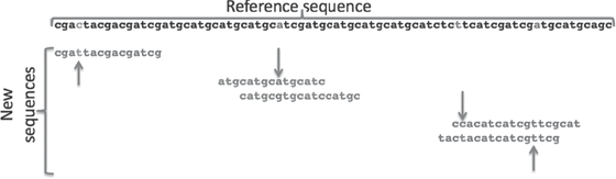
Figure 8.2 SNP ascertainment. The reference sequence is shown at the top. Three areas where sequences match the reference sequence are shown. The fragments on the left and middle have one potential SNP each, while the sequence on the right has two potential SNPs. The upward arrows indicate SNPs that are not ascertained, while downward arrows indicate SNPs that are ascertained and used in further research. See plate 6.
Ascertainment of SNPs for Human Origins Studies
| Ascertainment panel |
Sequencing depth |
Candidate SNPs |
Phase 2 valid |
| 1. French |
4.4 |
333,492 |
111,970 |
| 2. Han |
3.8 |
281,819 |
78,253 |
| 3. Papuan1 |
3.6 |
312,941 |
48,531 |
| 4. San |
5.9 |
548,189 |
163,313 |
| 5. Yoruba |
4.3 |
412,685 |
124,115 |
| 6. Mbuti |
1.2 |
39,178 |
12,162 |
| 7. Karitiana |
1.1 |
12,449 |
2,635 |
| 8. Sardinian |
1.3 |
40,826 |
12,922 |
| 9. Melanesian |
1.5 |
51,237 |
14,988 |
| 10. Cambodian |
1.7 |
53,542 |
16,987 |
| 11. Mongolian |
1.4 |
35,087 |
10,757 |
| 12. Papuan2 |
1.4 |
40,996 |
12,117 |
| 13. Denisova-San |
* |
418,841 |
151,435 |
| Unique SNPs total |
|
181,2990 |
542,399 |
Source: From Patterson et al. 2012, supplemental table 3.
Ascertainment is tricky business. What it does is set a baseline for variation studies in human genetics. If you do it incorrectly, or in a biased fashion, problems can arise; and in 2013 Joseph Lachance and Sarah Tishkoff suggested that ascertainment problems can cause genotyping arrays to contain biased sets of pre-ascertained SNPs. Emily McTavish and David Hillis have studied the problem of ascertainment bias in animal populations, finding that two types of bias may result from ascertainment problems. The first is what is known as minor allele frequency bias. This bias can result in overrepresentation of SNPs that have high minor allele frequencies and in underrepresentation of SNPs that have low minor allele frequencies. This kind of bias will influence which SNPs are put onto a chip for analysis, and entire categories of SNPs that might influence the analysis are excluded for this reason. The second kind of bias concerns the number of individuals in an ascertainment group or subpopulation. This parameter will influence the lower limit of frequencies of alleles in populations, so that SNPs that exist in low frequencies are unlikely to be observed in an ascertainment group. This many impact inference from study results. For example, it has been argued that low-frequency alleles may be the result of recent mutations that are limited to specific geographic areas simply because they have not had time to move around. If the ascertainment bias is against these SNPs, then extra information on geographic clustering of alleles for the SNP would be excluded from the study. If, on the other hand, those low-frequency SNPs were biased for a panel, then more geographic clustering would be inferred than warranted.
Because of these uncertainties, the answer to any question one might ask without a fully objective set of SNPs may be biased, because while the SNPs selected for the array or the targeted data set may be chosen for reasons that are fully in line with the research question, they may not be applicable to subsequent research questions. What this means is that we need to be very careful about the actual research questions we ask and how we approach answering them. This is key when we are looking at questions about human origins and history, for it is imperative to exclude the “ascertainment bias” that results from any inadequacies in the ascertainment process.
To drive this point home, consider the establishment of what human geneticists call “ancestral informative markers” (AIMs). In human genomics, these markers are supposedly fixed SNPs that differentiate between specific populations. To us, however, AIMs are the result of an extreme ascertainment process, as described in figure 8.3.
A final cautionary tale involves a recent study on the genetics of Europeans that gained a lot of press when it was first published, particularly because of its claim that the authors could identify individuals to within several hundred kilometers of their birthplace. In 2008, John Novembre and colleagues conducted a genome-level study by developing a panel of markers for different European populations. The procedure used was complicated, and the markers they eventually used are best described as AIMs for different subpopulations of Europeans. The way in which these markers were “ascertained” is illuminating. Table 8.3 shows the “trimming” process the Novembre group used to arrive at their set of markers and demonstrates how the strategic removal of individuals can lead to a preconceived notion of genomic differentiation among these European subpopulations. After the trimming, the researchers had removed nearly 800 out of 3,200 individuals. In other words, 25 percent of the individuals were rejected because they were “outliers.” As if this were not enough, for ease of computation another one thousand or so individuals were removed to further reduce the data set, eliminating individuals with genome sequences apparently related to others in the sample.
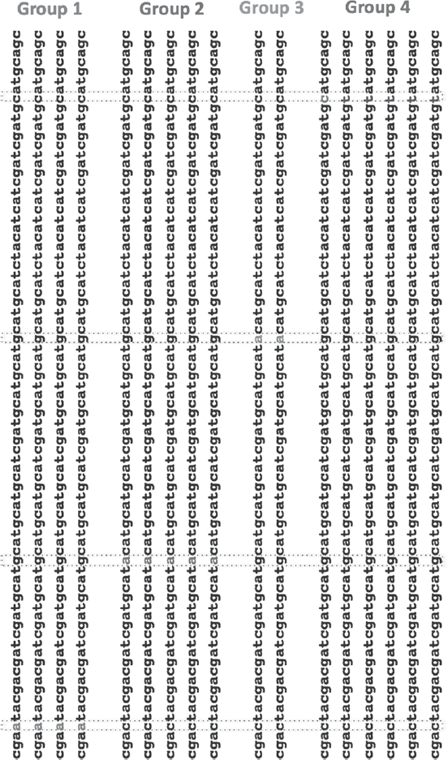
Figure 8.3 Finding AIMs in genetic data. The populations or groups are predetermined using some criterion. The sequences are then scanned for fixed and different SNPs that can be used as diagnostics. The diagnostic in group 1 is an “a” in position 4; in group 2 it is an “a” in position 20; in group 3 it is an “a” in position 40; and in group 4 it is a “t” in position 60. See plate 7.
Exclusion Strategies and Effect on Data Set Size in an AIM Study
| Sample size |
Stage of analysis |
| 3,192 |
Total individuals of purported European descent |
| 2,933 |
After exclusion of individuals with origins outside Europe |
| 2,409 |
After exclusion of individuals with mixed grandparental ancestry |
| 2,385 |
After exclusion of putative related individuals |
| 2,351 |
After exclusion based on preliminary run |
We suggest that removing outliers in this way causes researchers to miss something incredibly important about the genetics of human populations. Sure, when you cherry-pick a data set you will obtain a neat answer that agrees well with the rules under which you did your cherry-picking. But the really interesting aspect of the Novembre group’s study is actually the 25 percent of the population that was left out. Because what does an “outlier” really mean here? In the real world, outliers are most likely migrants or admixed people. The large proportion of individuals (a quarter!) who fall into this category is very significant in and of itself; and the actual proportion may in fact even be larger than indicated in this study, because many of the 1,300 or so individuals left at the end of the trimming process could be removed using similar procedures to make the results even cleaner. Indeed, it turns out that to get a geographical assignment within 800 kilometers with 99 percent accuracy, you would have to remove another six hundred or so “outliers.” And this, of course, would place about half of the population in the interesting category of people who have migrated or admixed. To us, this aspect of the variation observed is by far the more interesting part and gives us a much better description of reality.
Finally, it seems highly probable that, under current demographic trends, the structure that Novembre and his colleagues were striving to document in human populations is fated to erode even further in the next few centuries (should our species make it that long). Consequently, we profoundly doubt the utility of structured analysis as a way of usefully describing human populations over the long term. We will return to these approaches in detail when we describe the pitfalls of clustering.